
AI research workflow
One click to complete your research workflow from your handwritten concept
Upload your handwritten concept. EasySeer validates the concept, writes the code, runs it, drafts the manuscript, formats the paper and delivers it. You review every step.
A narrated 2-minute tour of the real tool. Open the full product tour →
Samples
Two sample projects, from input to paper
Two real deliveries. Pick a project, then step through all six stages: the inputs, the generated code, the run, every result, the manuscript in a PDF viewer and the formatted IEEE paper. Click any page or graph to enlarge it.
Loading the PDF… 0%
Everything starts from the concept document, together with the proposal, base papers and datasets in one project folder. Each is read and scored before anything is written.
- Concept PDF, 9 handwritten pages
- Proposal DOCX
- Base papers, 16 PDFs
- FruitNet and FruitQ datasets
The concept document is the starting point. Scroll through all 9 handwritten pages in the viewer.
"""MLRI-Net project hub (tkinter GUI).

* "Run Full Pipeline & Show Graphs" runs every stage for the selected dataset(s)
  on a background thread, then shows all graphs in the built-in gallery.
* Every stage can also be run on its own, as can the sample case study, the
  self-checks and the demo.
* Settings (data percentage, per-class cap, epochs, ...) are saved to run_settings.json.

Start:  python main.py
"""
import os
import queue
import random
import subprocess
import sys
import threading
import tkinter as tk
import traceback
from pathlib import Path
from tkinter import messagebox, scrolledtext, ttk

from PIL import Image, ImageTk

import run_config as cfg
from data_loader import discover_datasets
from feature_cache_builder import PipelineCancelled
from full_pipeline_runner import STAGE_ORDER, STAGE_TITLES, run_full_pipeline
from project_paths import (CODE_DIR, EXPERIMENTAL_OUTPUT_DIR, PARAMETERS_DIR, RESULTS_DIR, SAMPLE_CASE_STUDY_DIR,
                           ensure_output_folders)

ACCENT = "#882255"
PANEL_BG = "#F7F4F2"
THUMB = 230


def open_folder(path):
    path = Path(path)
    path.mkdir(parents=True, exist_ok=True)
    if sys.platform.startswith("win"):
        os.startfile(str(path))                                  # noqa: S606 (Windows only)
    elif sys.platform == "darwin":
        subprocess.Popen(["open", str(path)])
    else:
        subprocess.Popen(["xdg-open", str(path)])


class GraphGallery(ttk.Frame):
    """Scrollable grid of result graphs; click a thumbnail to enlarge it."""

    def __init__(self, master):
        super().__init__(master)
        top = ttk.Frame(self)
        top.pack(fill="x", pady=(4, 2))
        ttk.Label(top, text="Show:").pack(side="left", padx=(6, 2))
        self.filter = ttk.Combobox(top, state="readonly", width=34)
        self.filter.pack(side="left")
        self.filter.bind("<<ComboboxSelected>>", lambda _e: self.refresh())
        ttk.Button(top, text="Reload graphs", command=self.refresh).pack(side="left", padx=6)
        self.count_label = ttk.Label(top, text="")
        self.count_label.pack(side="left", padx=6)
        self.canvas = tk.Canvas(self, background="white", highlightthickness=0)
        scroll = ttk.Scrollbar(self, orient="vertical", command=self.canvas.yview)
        self.inner = tk.Frame(self.canvas, background="white")
        self.inner.bind("<Configure>", lambda _e: self.canvas.configure(scrollregion=self.canvas.bbox("all")))
        self.canvas.create_window((0, 0), window=self.inner, anchor="nw")
        self.canvas.configure(yscrollcommand=scroll.set)
        self.canvas.pack(side="left", fill="both", expand=True)
        scroll.pack(side="right", fill="y")
        self.canvas.bind_all("<MouseWheel>", lambda e: self.canvas.yview_scroll(int(-e.delta / 120), "units"))
        self.canvas.bind_all("<Button-4>", lambda _e: self.canvas.yview_scroll(-1, "units"))
…
"""Proposed method - MLRI-Net (Mean Squared LogCosh loss based Residual Inception Network).
Pipeline (context.docx Sec. 3): CIEWF -> DLNet -> CutMix/MixUp -> {f1 CS-LMP, f2 ResNeXt-101}
-> MLRI-Net -> fruit type + fruit grade -> XAI.
Architecture (Sec. 3.6):
image branch : segmented image Sm (128x128) -> frozen ResNet18 conv1..layer3 (cached)
-> trainable layer4 -> SE channel attention (residual) -> inception (1024 ch) -> GAP
fusion : [1024 image | 256 from f1 CS-LMP | 256 from f2 ResNeXt-101] = 1536-D
heads : FC1 (1024) -> FC2 (128) -> fruit-type head and grade head
loss : L_Tot = 0.5 RMSLE + 0.5 LogCosh on softmax outputs, summed over both heads
optimiser : Adam (beta1 0.9, beta2 0.999, eps 1e-8), lr 1e-3, ReduceLROnPlateau, early stopping
Ablation variants (Sec. 4.7.2) reuse the class with a different configuration:
without DLNet -> image branch, f1 and f2 computed on the CIEWF image (no background isolation)
without augmentation -> no CutMix / MixUp
"""
import torch
import torch.nn as nn
import run_config as cfg
from comparison_method_interface import NeuralTwoHeadMethod
from loss_rmsle_logcosh import MeanSquaredLogCoshLoss
from rai_net_blocks import RAIImageBranch, TwoHeadClassifier
from texture_features_cslmp import CSLMP_DIM
class MLRINet(nn.Module):
def __init__(self, n_types, n_grades, cslmp_dim=CSLMP_DIM, resnext_dim=1000, proj=256, dropout=None):
super().__init__()
dropout = cfg.DROPOUT if dropout is None else dropout
self.image_branch = RAIImageBranch()
self.cslmp_proj = nn.Sequential(nn.Linear(cslmp_dim, proj), nn.ReLU(inplace=True), nn.Dropout(dropout))
self.resnext_proj = nn.Sequential(nn.Linear(resnext_dim, proj), nn.ReLU(inplace=True), nn.Dropout(dropout))
self.classifier = TwoHeadClassifier(RAIImageBranch.out_dim + 2 * proj, n_types, n_grades,
fc1=1024, fc2=128, dropout=dropout)
def forward(self, layer3_maps, vectors, return_maps=False):
f1, f2 = vectors
if return_maps:
image_vec, maps = self.image_branch(layer3_maps, return_maps=True)
else:
image_vec = self.image_branch(layer3_maps)
fused = torch.cat([image_vec, self.cslmp_proj(f1), self.resnext_proj(f2)], dim=1)
type_logits, grade_logits, embedding = self.classifier(fused)
if return_maps:
return type_logits, grade_logits, embedding, maps
return type_logits, grade_logits, embedding
class MLRINetMethod(NeuralTwoHeadMethod):
key = "mlri_net"
display_name = "MLRI-Net (proposed)"
source = "Proposed method (context.docx Sec. 3)"
map_key = "layer3_seg"
vector_keys = ("cslmp_seg", "resnext_seg")
augment = "mix"
default_batch_size = None # -> run_config.BATCH_SIZE at run time
def build_model(self):
return MLRINet(self.n_types, self.n_grades)
def build_optimizer(self, model):
params = [p for p in model.parameters() if p.requires_grad]
return torch.optim.Adam(params, lr=cfg.LEARNING_RATE, betas=(cfg.ADAM_BETA1, cfg.ADAM_BETA2),
eps=cfg.ADAM_EPSILON)
def loss(self):
return MeanSquaredLogCoshLoss()
…"""Building blocks of RAI-Net (Residual-Attention-Inception Network).
Source: Maurya et al., "RAI-Net: Tomato Plant Disease Classification Using
Residual-Attention-Inception Network" (IEEE Access 2025), Sec. IV, Fig. 2:
ResNet18 (fine-tuned last layers) -> 512x4x4 maps
-> channel attention (squeeze-and-excitation), applied residually: y_CA = CA(x) + x (Eq. 8)
-> inception module, concat of 1x1 | 1x1-3x3 | 1x1-5x5 | maxpool-1x1 (Eq. 9) -> 1024x4x4
-> global average pooling -> FC1 -> FC2 (128) -> classes
"""
import torch
import torch.nn as nn
from pretrained_backbones import pretrained_resnet18_layer4
class SqueezeExcitationAttention(nn.Module):
"""Eqs. (1)-(5): F_avg -> conv + ReLU -> conv -> sigmoid = M_c; F_hat = F * M_c."""
def __init__(self, channels=512, reduction=16):
super().__init__()
self.pool = nn.AdaptiveAvgPool2d(1)
self.reduce = nn.Conv2d(channels, channels // reduction, 1)
self.expand = nn.Conv2d(channels // reduction, channels, 1)
self.detach_gate = False # True while computing LRP (gate treated as constant)
def forward(self, x):
gate = torch.sigmoid(self.expand(torch.relu(self.reduce(self.pool(x)))))
if self.detach_gate:
gate = gate.detach()
return x * gate + x # Eq. (8): y_CA = CA(x) + x
def _conv_bn_relu(cin, cout, k):
return nn.Sequential(nn.Conv2d(cin, cout, k, padding=k // 2, bias=False),
nn.BatchNorm2d(cout), nn.ReLU(inplace=True))
class InceptionModule(nn.Module):
"""Eq. (9): multi-scale branches concatenated along channels (512 -> 1024)."""
def __init__(self, cin=512, branch=256):
super().__init__()
self.b1 = _conv_bn_relu(cin, branch, 1)
self.b3 = nn.Sequential(_conv_bn_relu(cin, branch // 2, 1), _conv_bn_relu(branch // 2, branch, 3))
self.b5 = nn.Sequential(_conv_bn_relu(cin, branch // 4, 1), _conv_bn_relu(branch // 4, branch, 5))
self.bp = nn.Sequential(nn.MaxPool2d(3, stride=1, padding=1), _conv_bn_relu(cin, branch, 1))
def forward(self, x):
return torch.cat([self.b1(x), self.b3(x), self.b5(x), self.bp(x)], dim=1)
class RAIImageBranch(nn.Module):
"""Trainable part of RAI-Net on top of the frozen layer3 maps (256x8x8 -> 1024-D)."""
out_dim = 1024
def __init__(self):
super().__init__()
self.layer4 = pretrained_resnet18_layer4() # residual blocks, ImageNet initialised
self.attention = SqueezeExcitationAttention(512)
self.inception = InceptionModule(512, 256)
self.pool = nn.AdaptiveAvgPool2d(1)
def forward(self, layer3_maps, return_maps=False):
l4 = self.layer4(layer3_maps)
att = self.attention(l4)
inc = self.inception(att)
pooled = torch.flatten(self.pool(inc), 1)
if return_maps:
return pooled, {"layer4": l4, "attention": att, "inception": inc}
…"""Stage 3.2 - Contextual Image Enhancement Wiener Filter (CIEWF).
Source: Sudhakar et al., "High-performance parallel multi-scale attention network
with explainable AI for intelligent diagnosis of leaf diseases in agricultural
systems", p. 5, Eqs. (1)-(3):
CIEWF[I(x1,x2)] = alpha + (beta^2 - beta_n^2) / beta^2 * (I(x1,x2) - alpha)
alpha = local mean over the surrounding window s
beta^2 = local variance over s, beta_n^2 = noise variance
This is a locally adaptive (Lee / Wiener) filter. In flat regions the local
variance is close to the noise variance, so the pixel is pulled to the local
mean (noise removed). On edges the variance is large, so the pixel is kept
(detail preserved). The paper says CIEWF "selects the most suitable window"
but gives no size, so each image is filtered with every candidate window in
CIEWF_WINDOWS and the window that removes the most noise while keeping at
least half of the edge energy is kept.
"""
import cv2
import numpy as np
from skimage.metrics import peak_signal_noise_ratio, structural_similarity
import run_config as cfg
def wiener_filter_channel(channel, window, noise_variance=None):
"""Apply Eq. (1) to one float channel in [0, 1]."""
alpha = cv2.blur(channel, (window, window)) # local mean, Eq. (2)
beta_sq = cv2.blur(channel * channel, (window, window)) - alpha ** 2 # local variance, Eq. (3)
beta_sq = np.maximum(beta_sq, 0.0)
if noise_variance is None: # beta_n^2 estimate
noise_variance = float(beta_sq.mean())
gain = np.maximum(beta_sq - noise_variance, 0.0) / np.maximum(beta_sq, noise_variance + 1e-12)
return alpha + gain * (channel - alpha)
def estimate_noise_sigma(gray):
"""Immerkaer's fast noise estimate (sigma) of a float grey image in [0, 1]."""
kernel = np.array([[1, -2, 1], [-2, 4, -2], [1, -2, 1]], dtype=np.float32)
conv = cv2.filter2D(gray.astype(np.float32), -1, kernel)
h, w = gray.shape
return float(np.sqrt(np.pi / 2.0) * np.abs(conv[1:-1, 1:-1]).sum() / (6.0 * (w - 2) * (h - 2)))
def _edge_energy(gray):
return float(cv2.Laplacian(gray.astype(np.float32), cv2.CV_32F).var()) + 1e-12
def enhance_image_ciewf(rgb_uint8, windows=None):
"""Enhance one RGB uint8 image. Returns (enhanced uint8, info dict)."""
windows = windows or cfg.CIEWF_WINDOWS
image = rgb_uint8.astype(np.float32) / 255.0
gray_in = cv2.cvtColor(image, cv2.COLOR_RGB2GRAY)
edge_in = _edge_energy(gray_in)
best = None
for window in windows:
out = np.stack([wiener_filter_channel(image[..., c], window) for c in range(3)], axis=-1)
out = np.clip(out, 0.0, 1.0)
gray_out = cv2.cvtColor(out, cv2.COLOR_RGB2GRAY)
noise = estimate_noise_sigma(gray_out)
edge_keep = _edge_energy(gray_out) / edge_in
# Prefer the lowest residual noise among windows that keep >= 50 % edge energy.
key = (edge_keep < 0.5, noise)
if best is None or key < best[0]:
best = (key, window, out, noise, edge_keep)
_, window, out, noise, edge_keep = best
enhanced = (out * 255.0 + 0.5).astype(np.uint8)
info = {
"ciewf_window": window,
"noise_sigma_before": estimate_noise_sigma(gray_in),
…EasySeer writes the project as separate Python files with a main program. Open any file, read it, and ask the chat what it does.
- In the project
- 48 Python files, plus requirements and a readme
- Shown
- The first lines of four real files
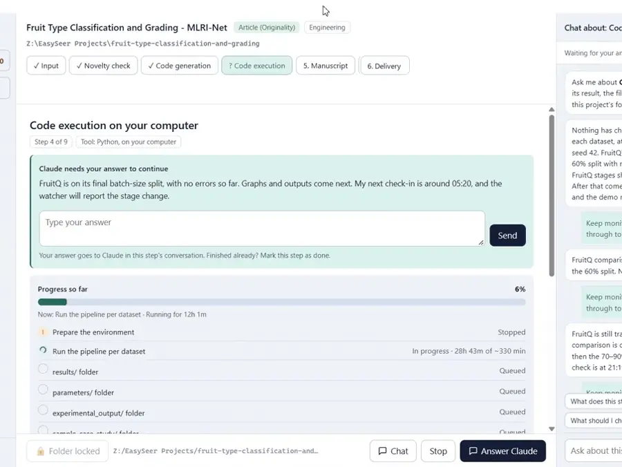
The code runs on your own computer. Every file, log and result is saved to the project folder, so nothing is hidden.
- Datasets
- FruitNet and FruitQ
- Compared with
- Five baseline methods
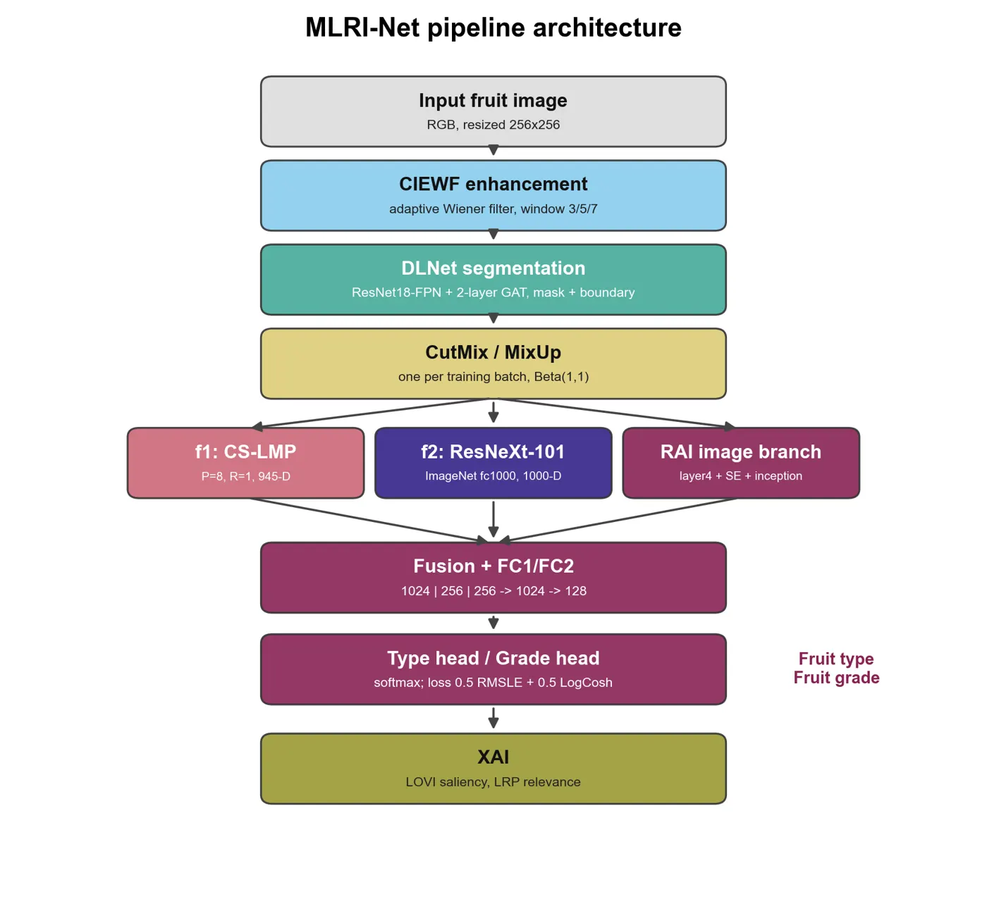
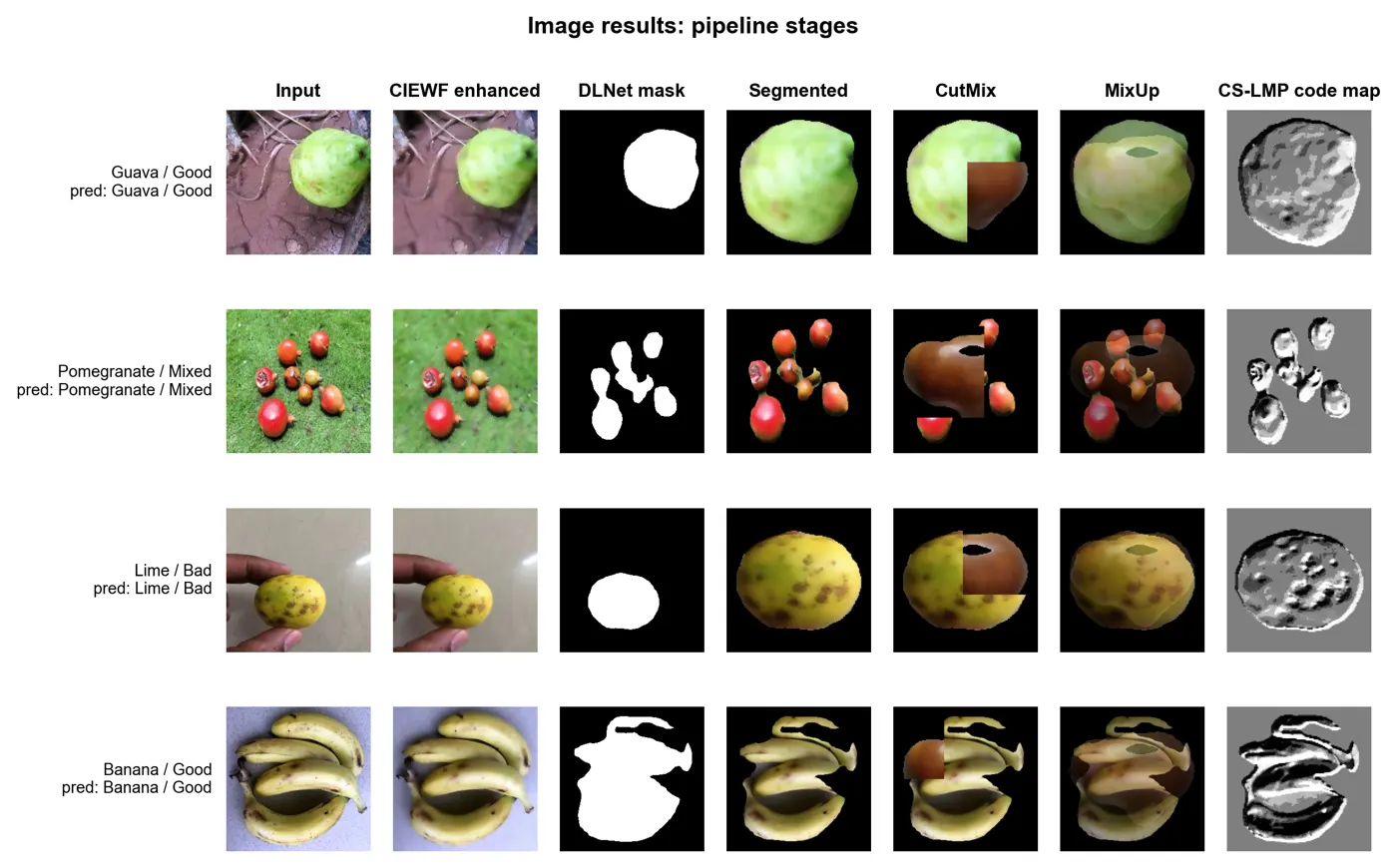
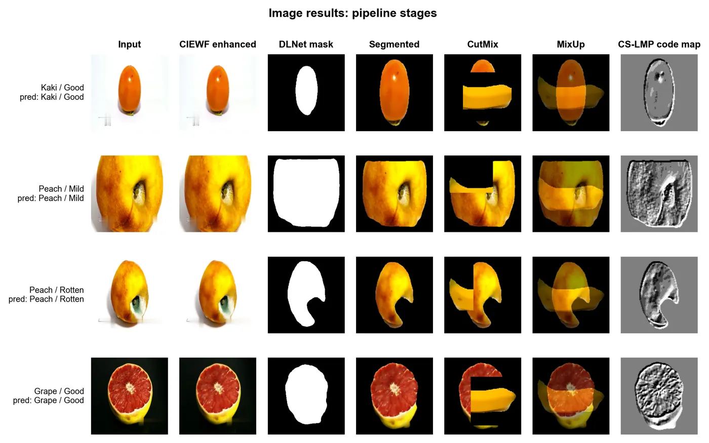
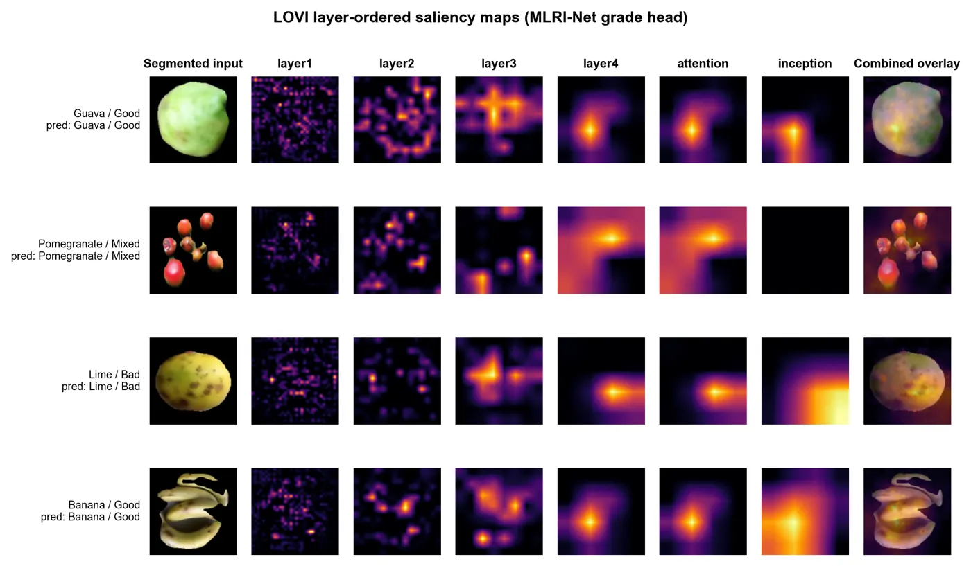
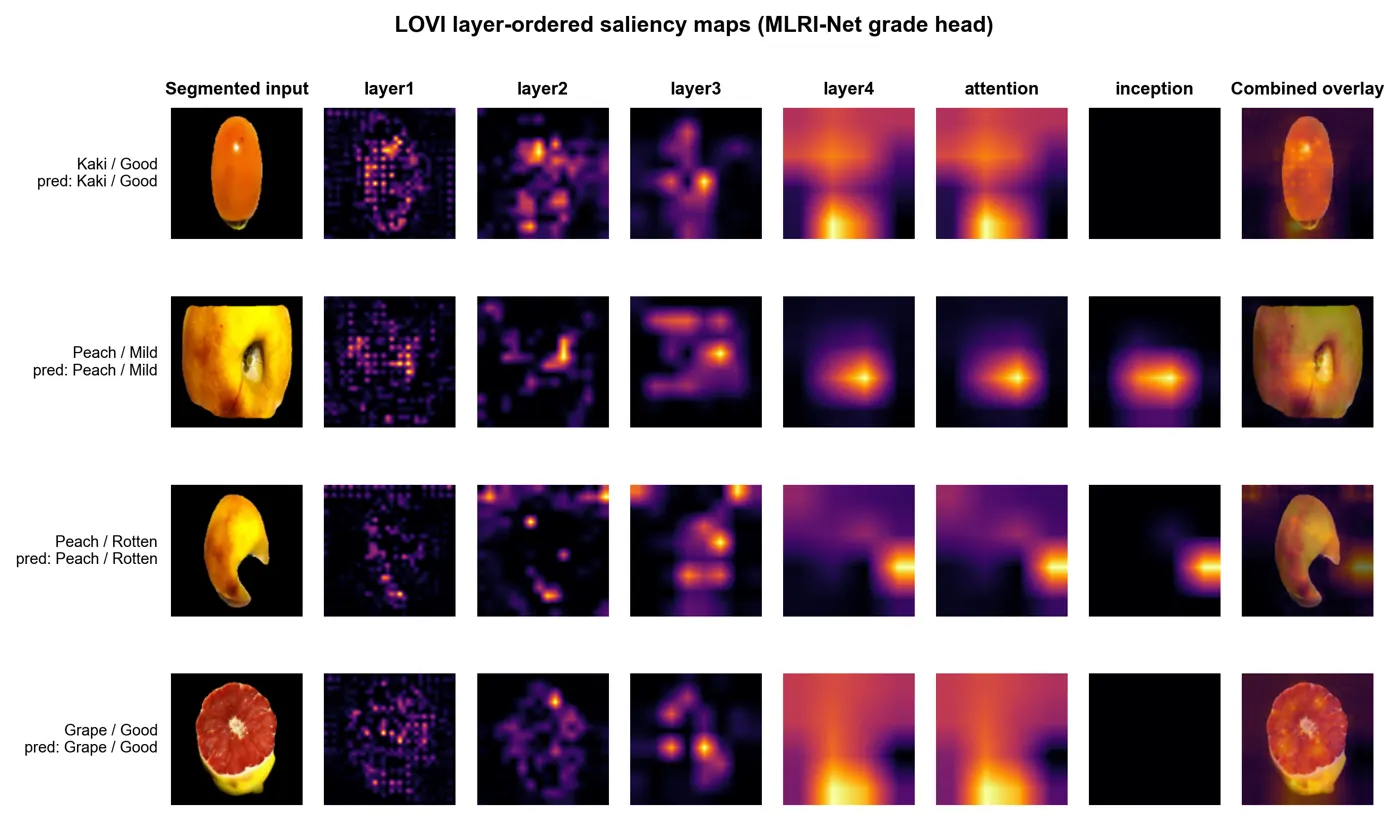
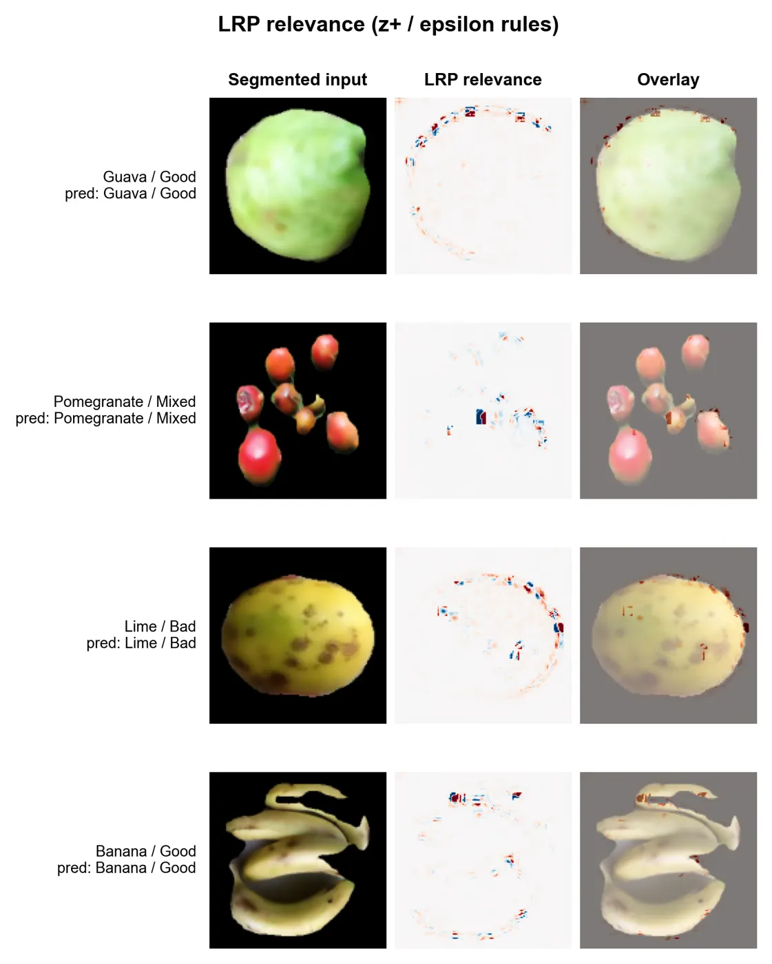
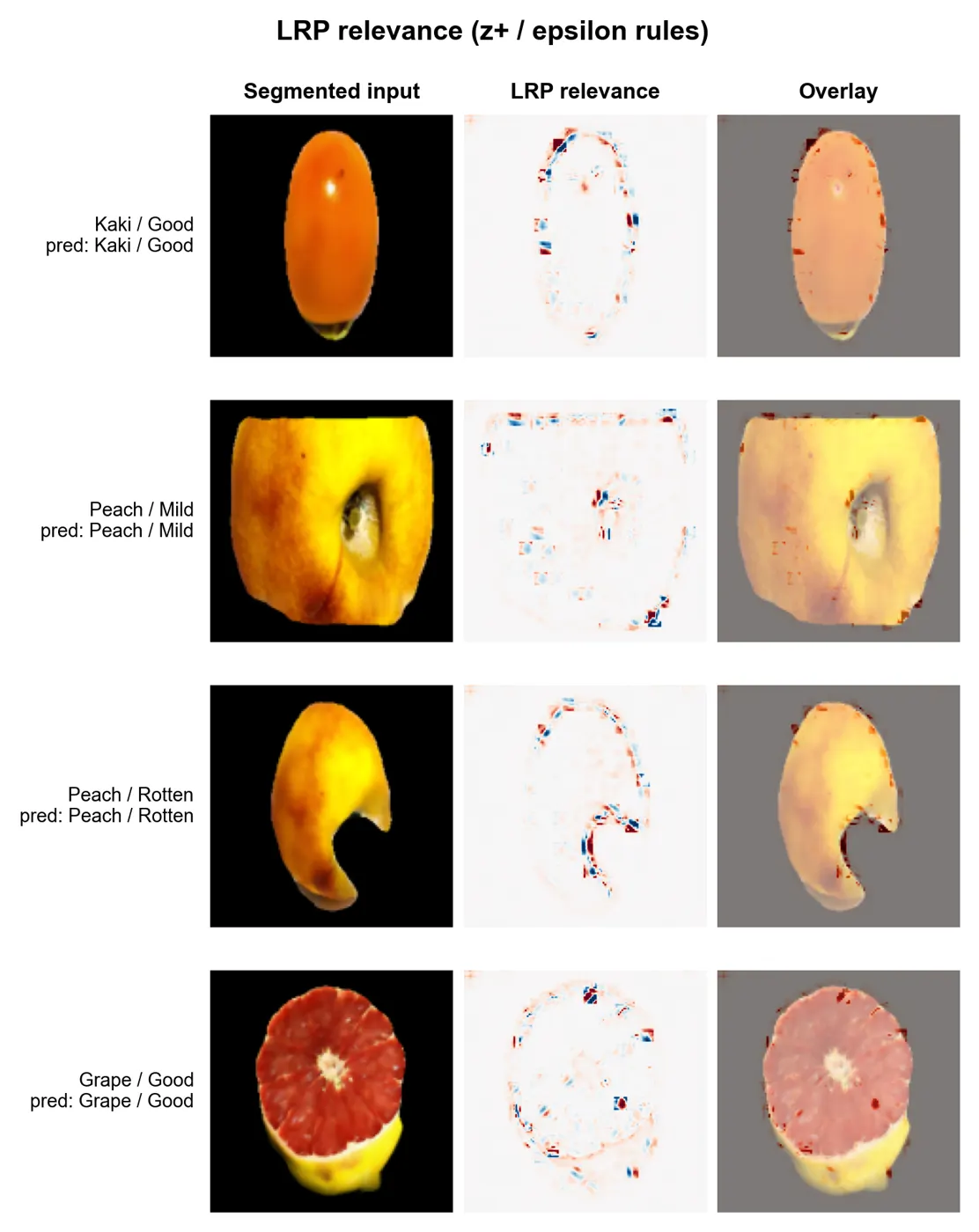
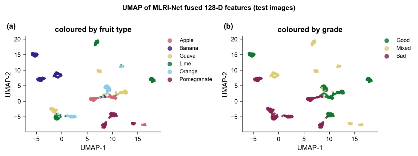
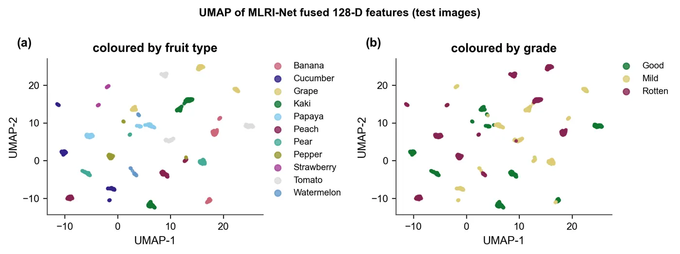
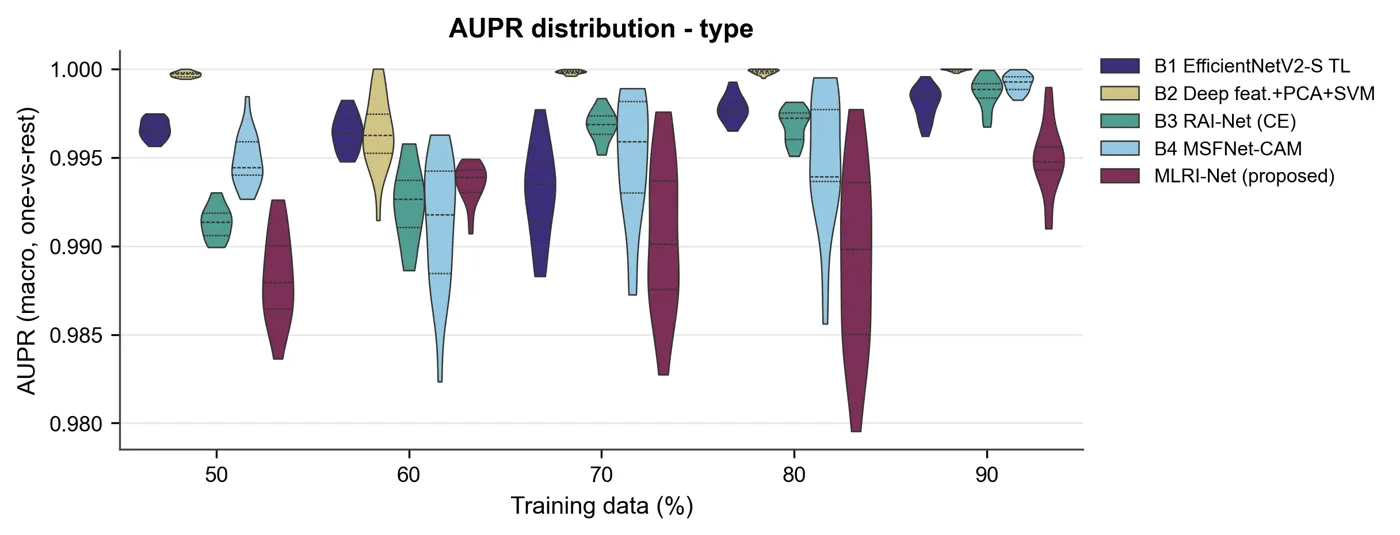
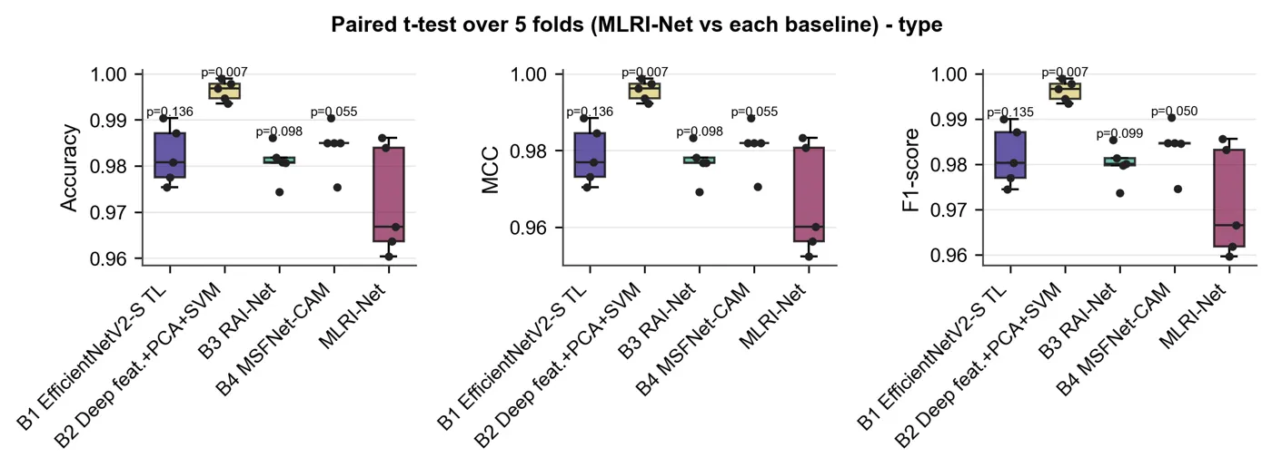
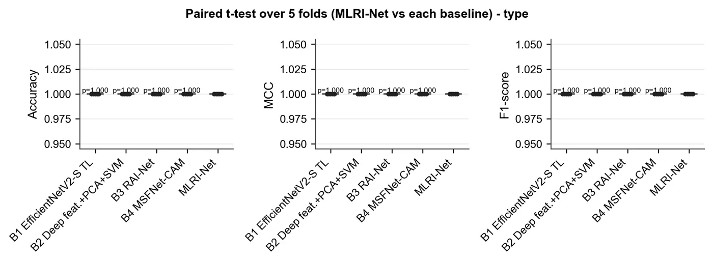
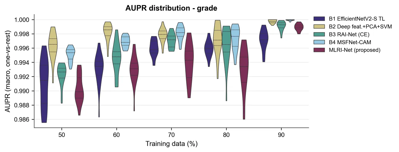
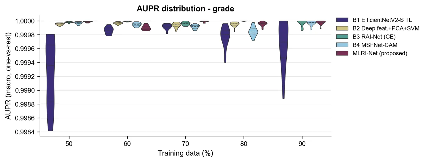
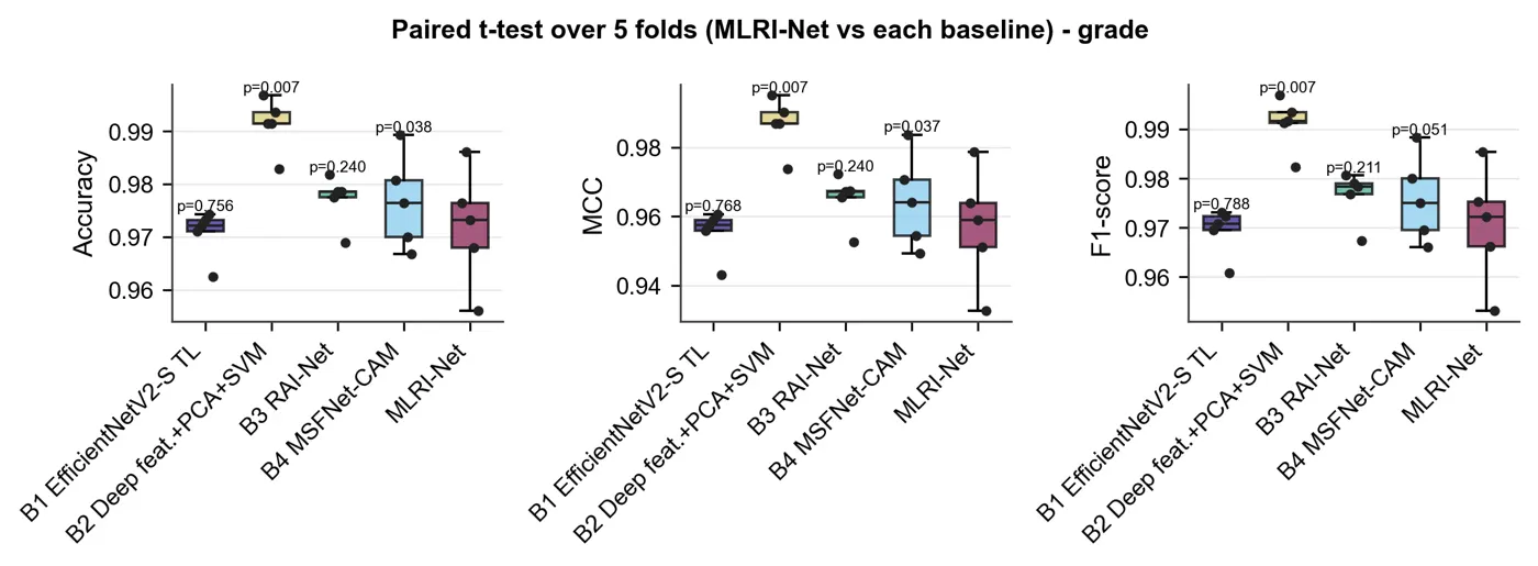
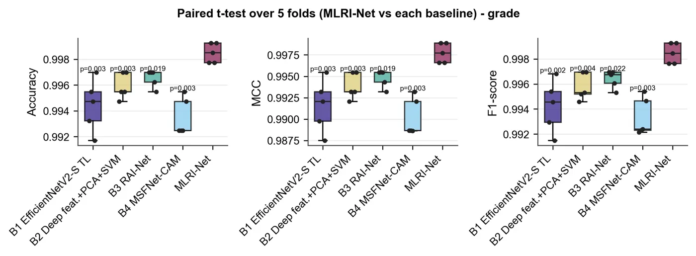
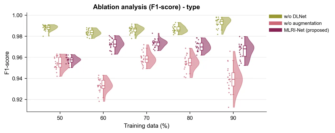
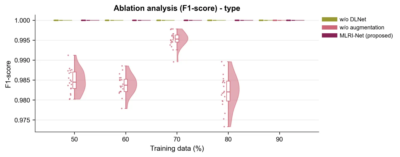
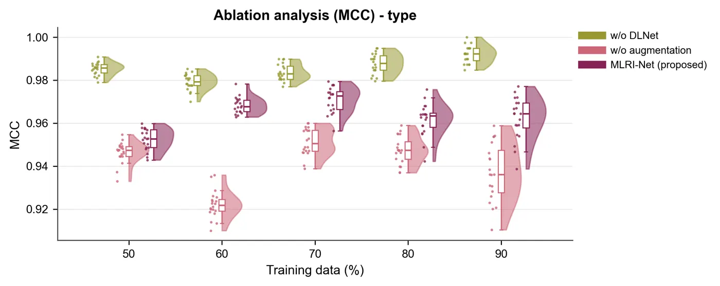
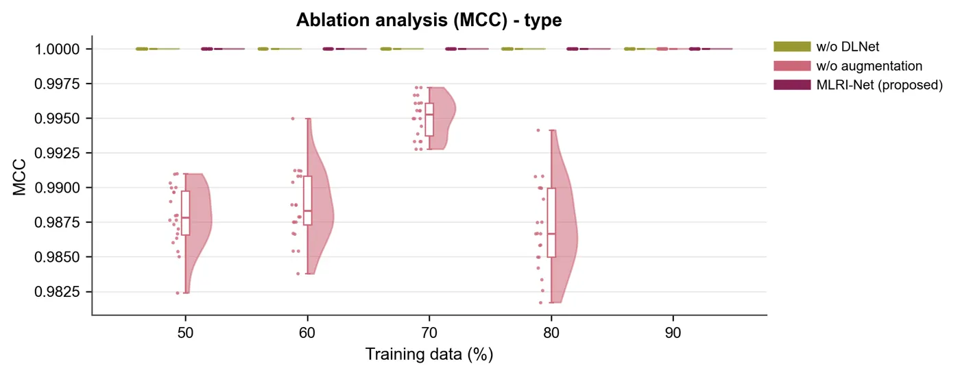
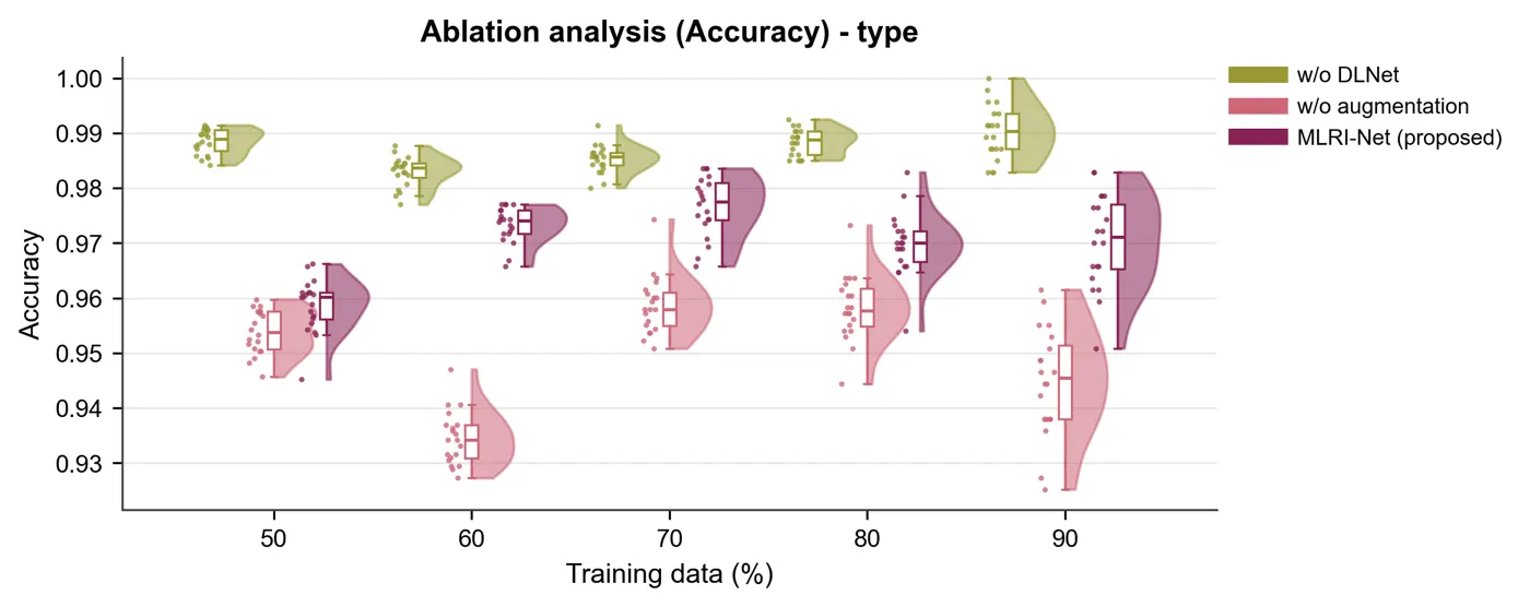
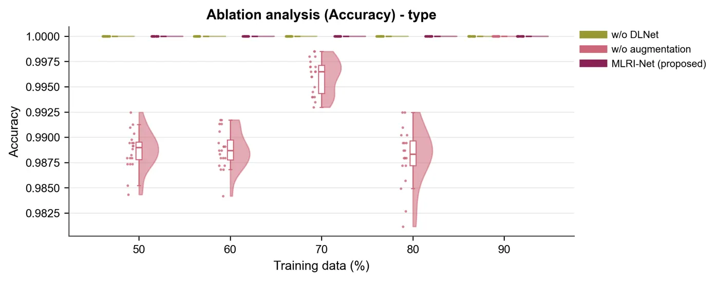
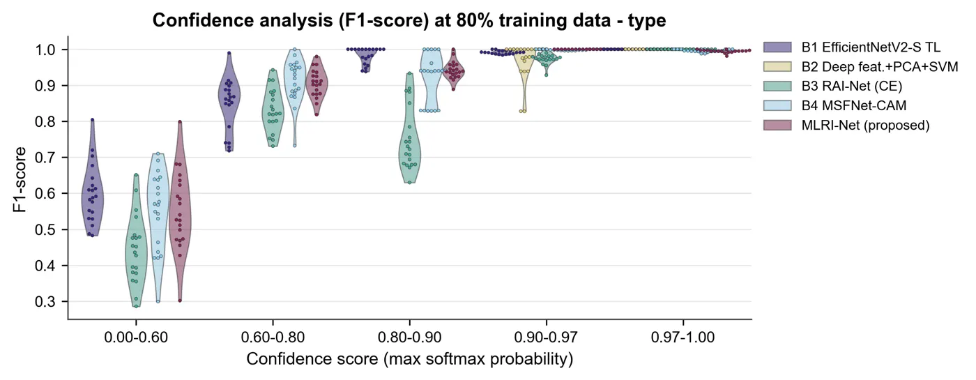
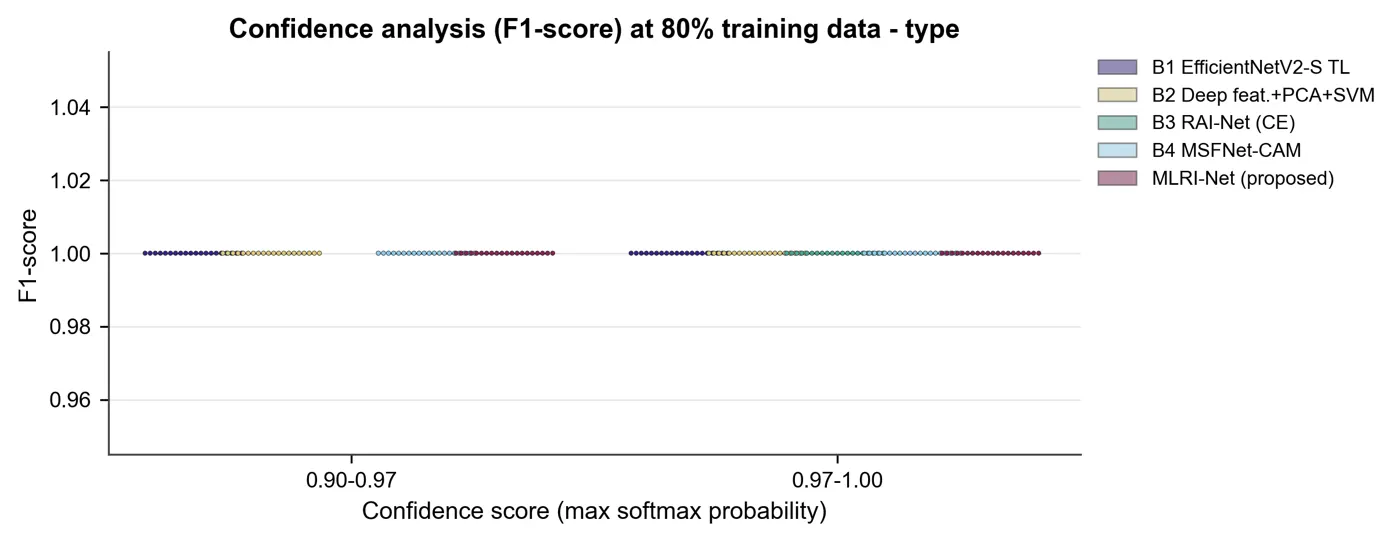
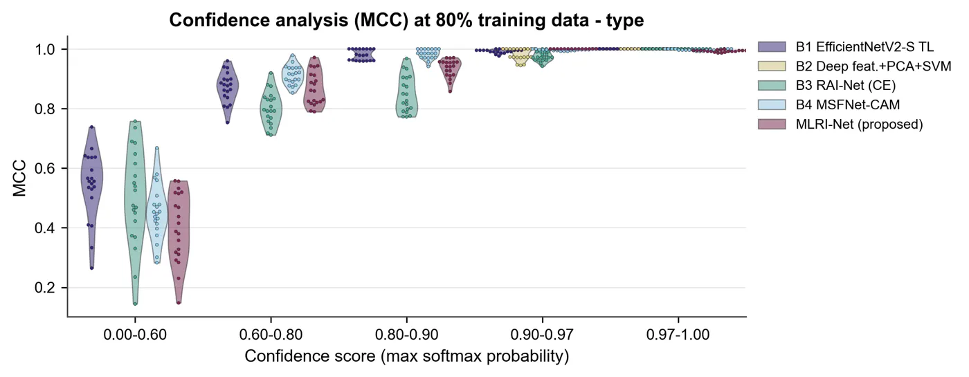
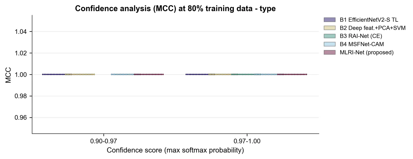
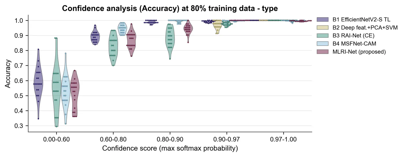
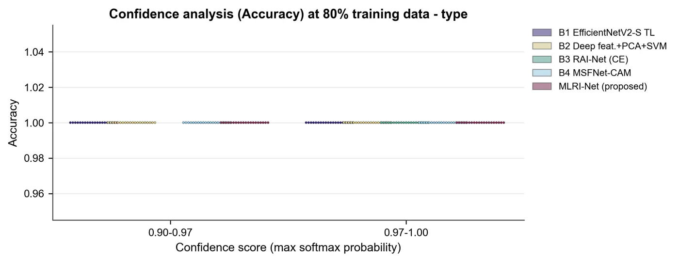
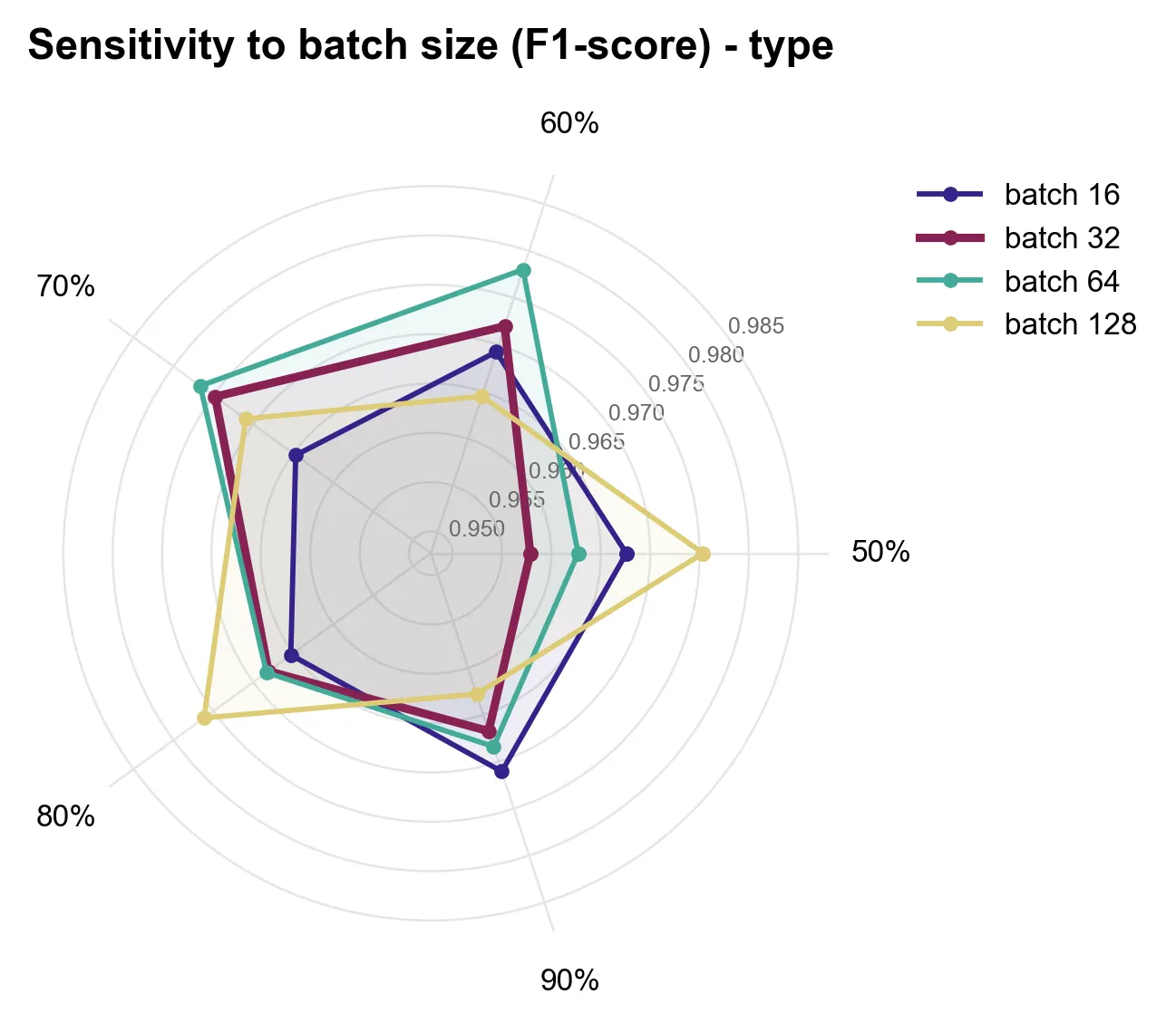
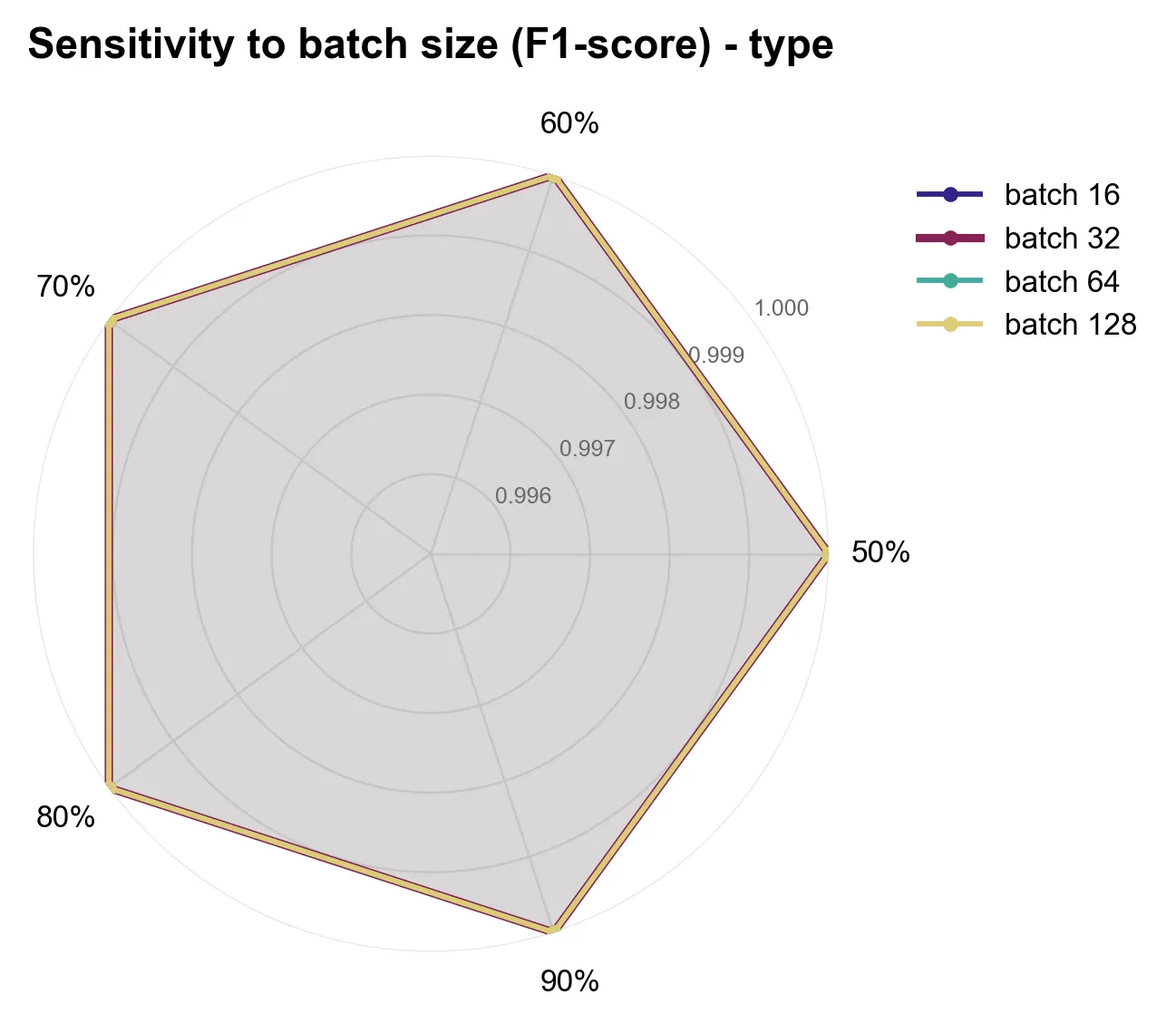
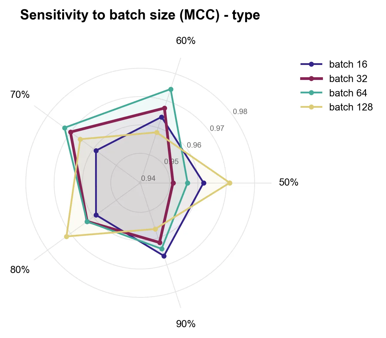
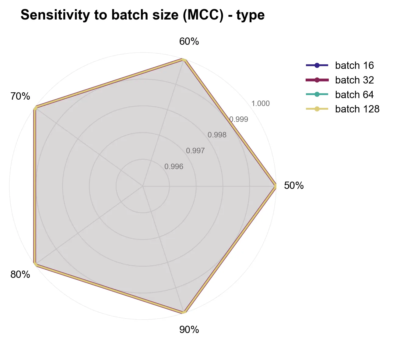
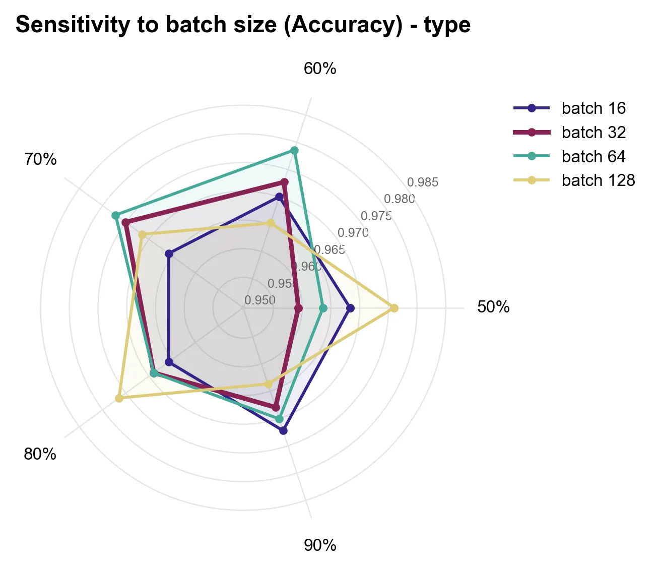
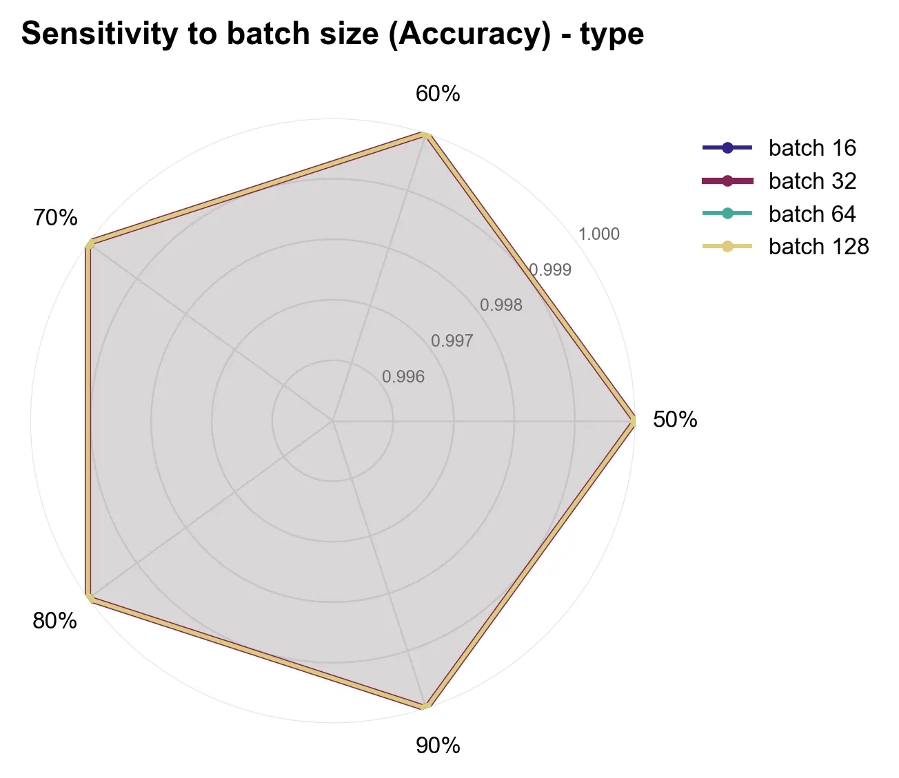
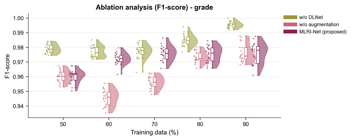
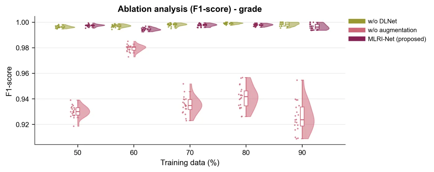
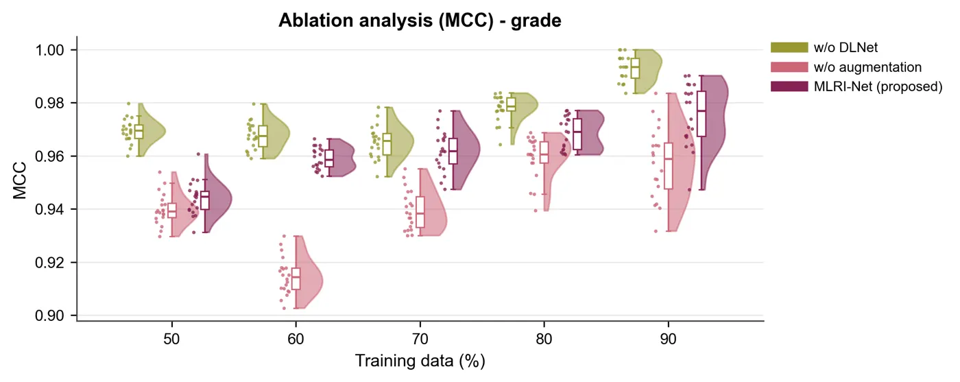
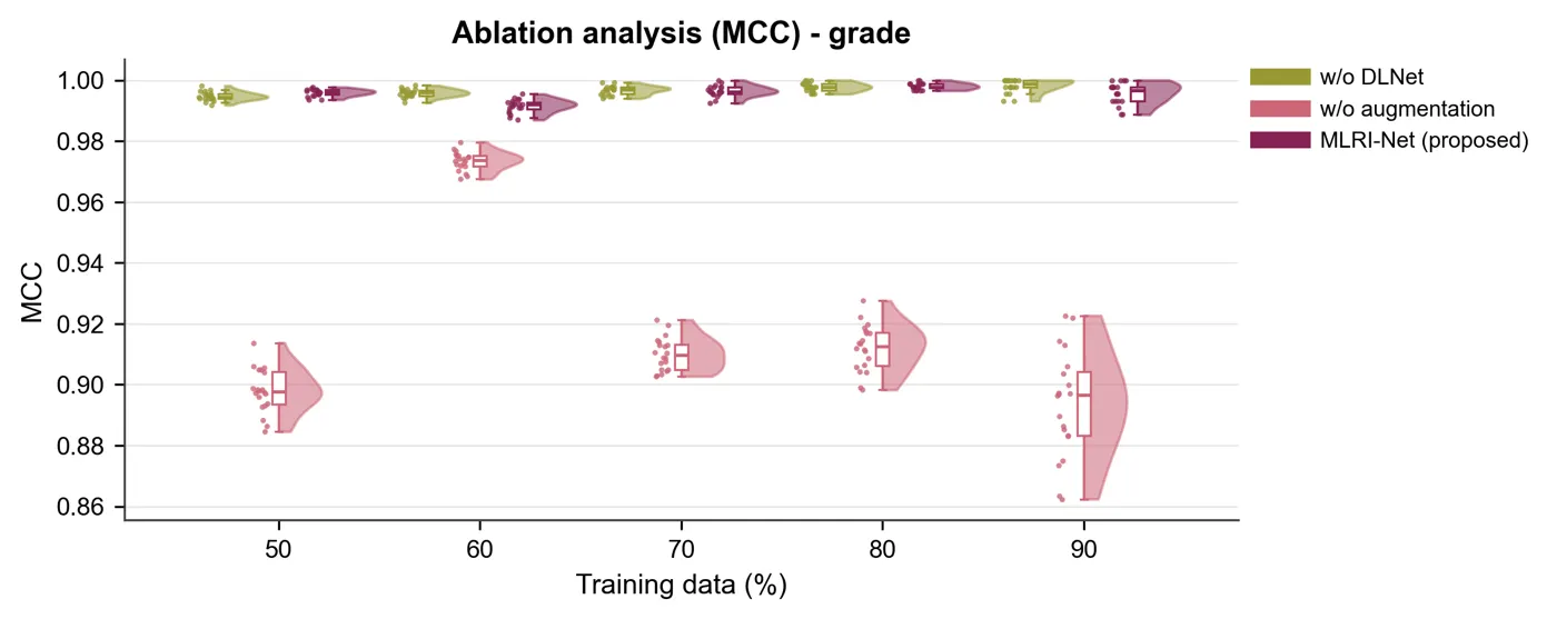
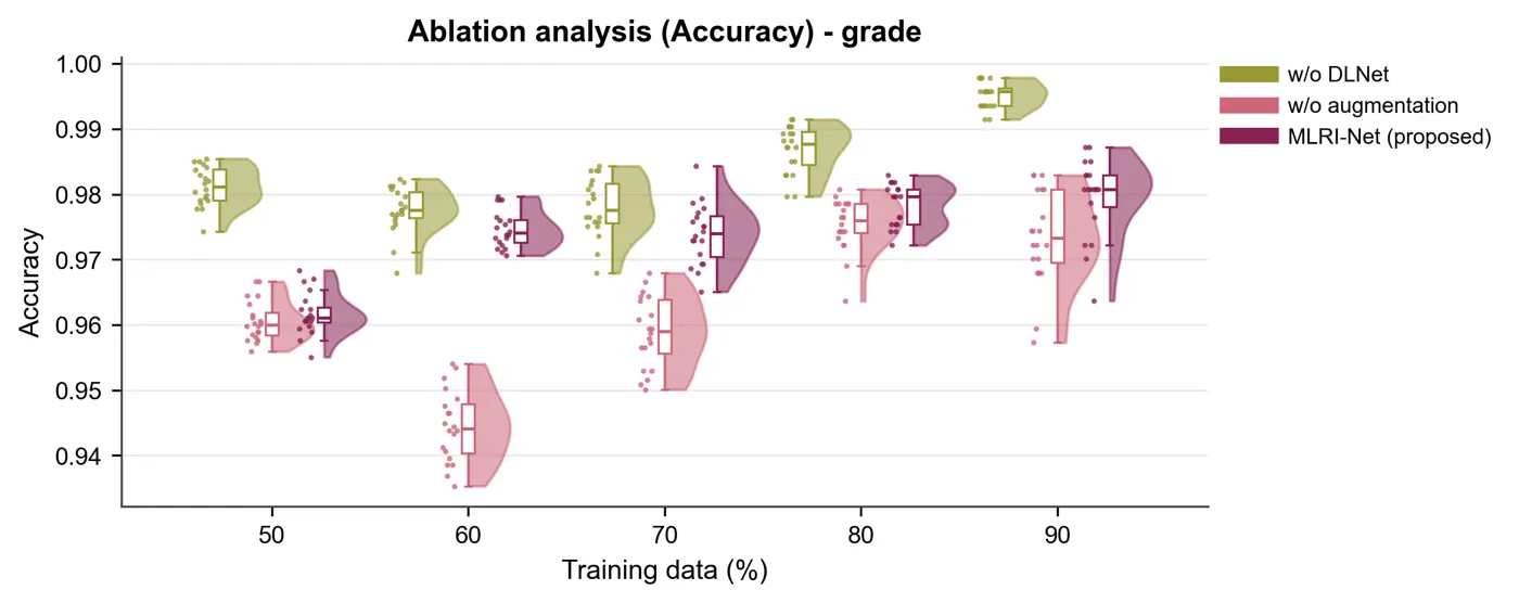
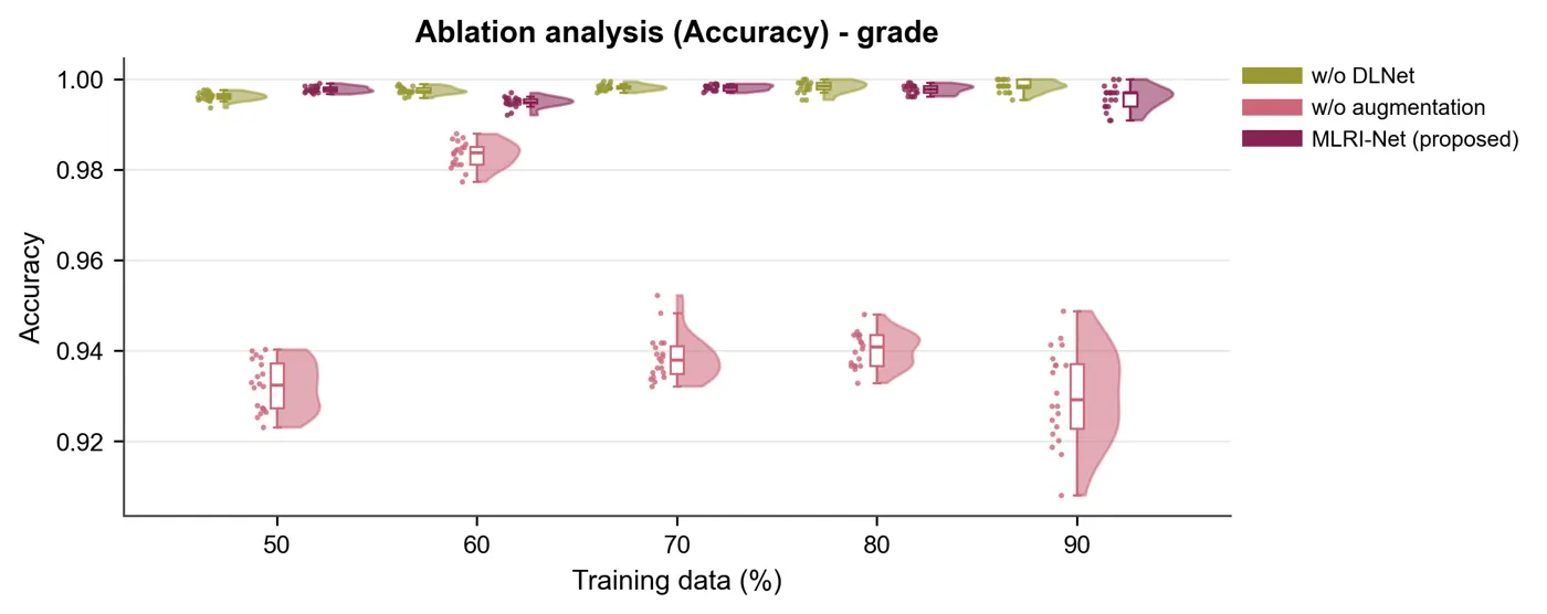
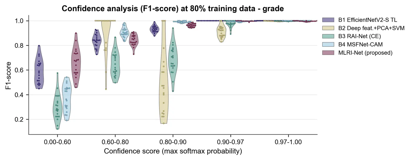
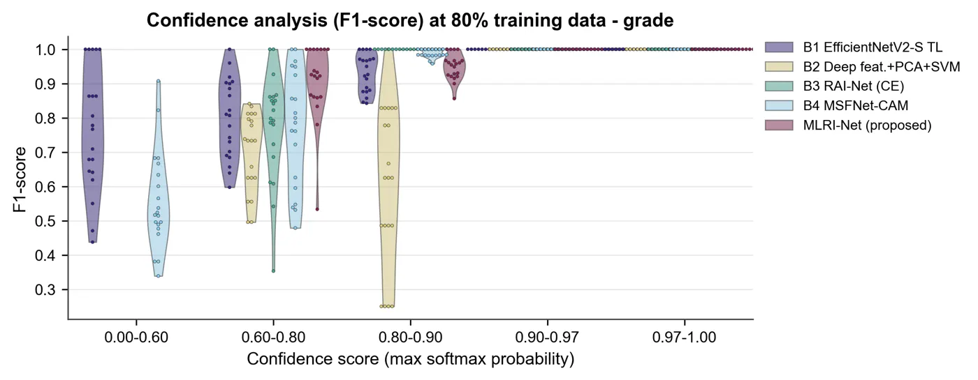
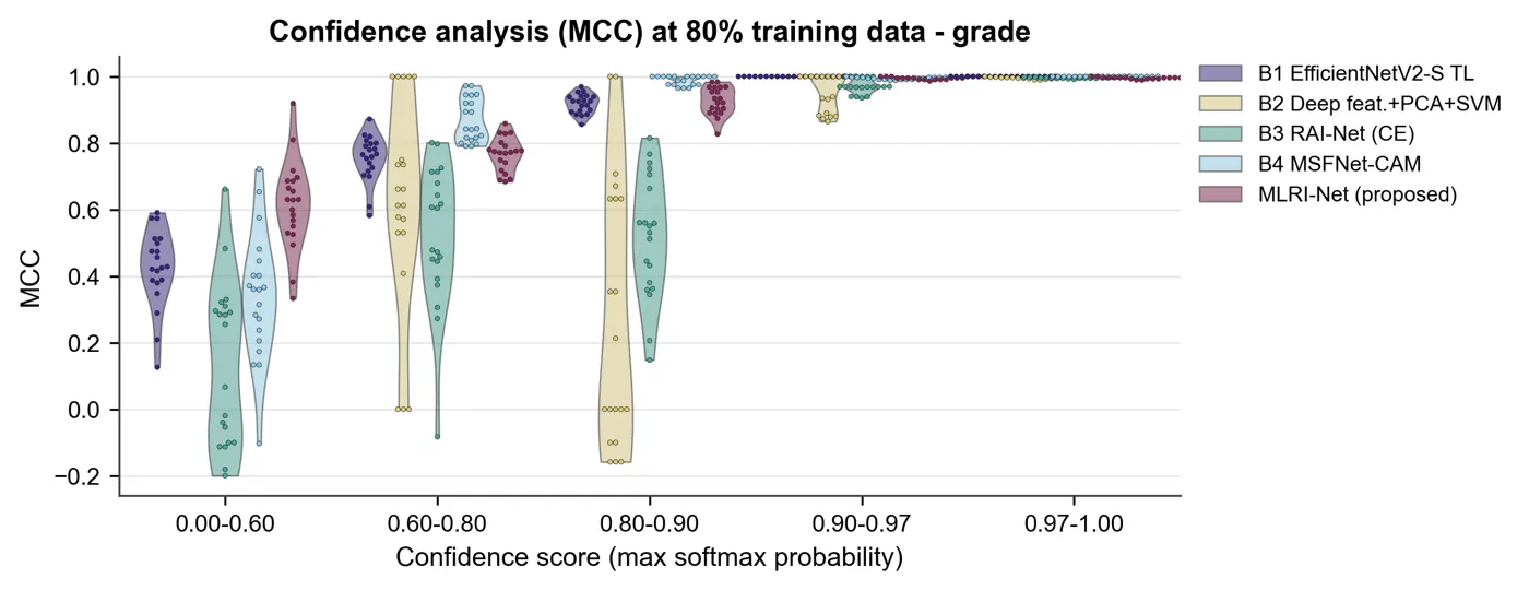
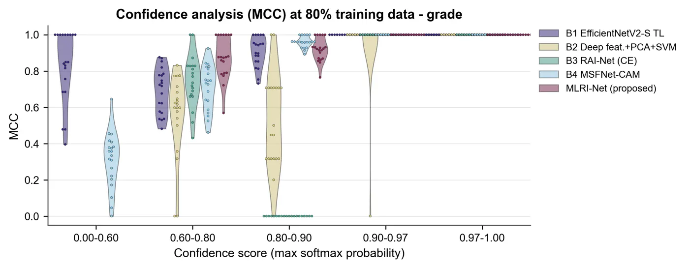
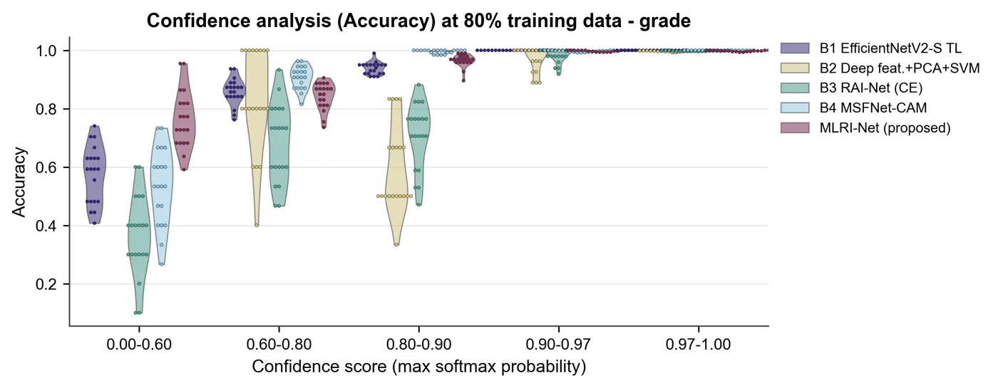
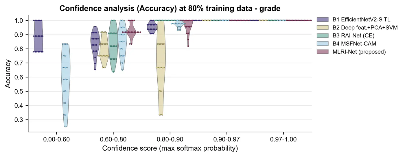
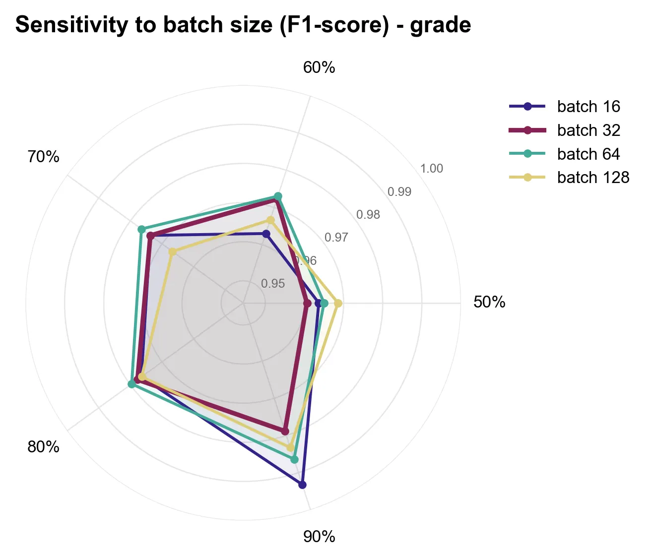
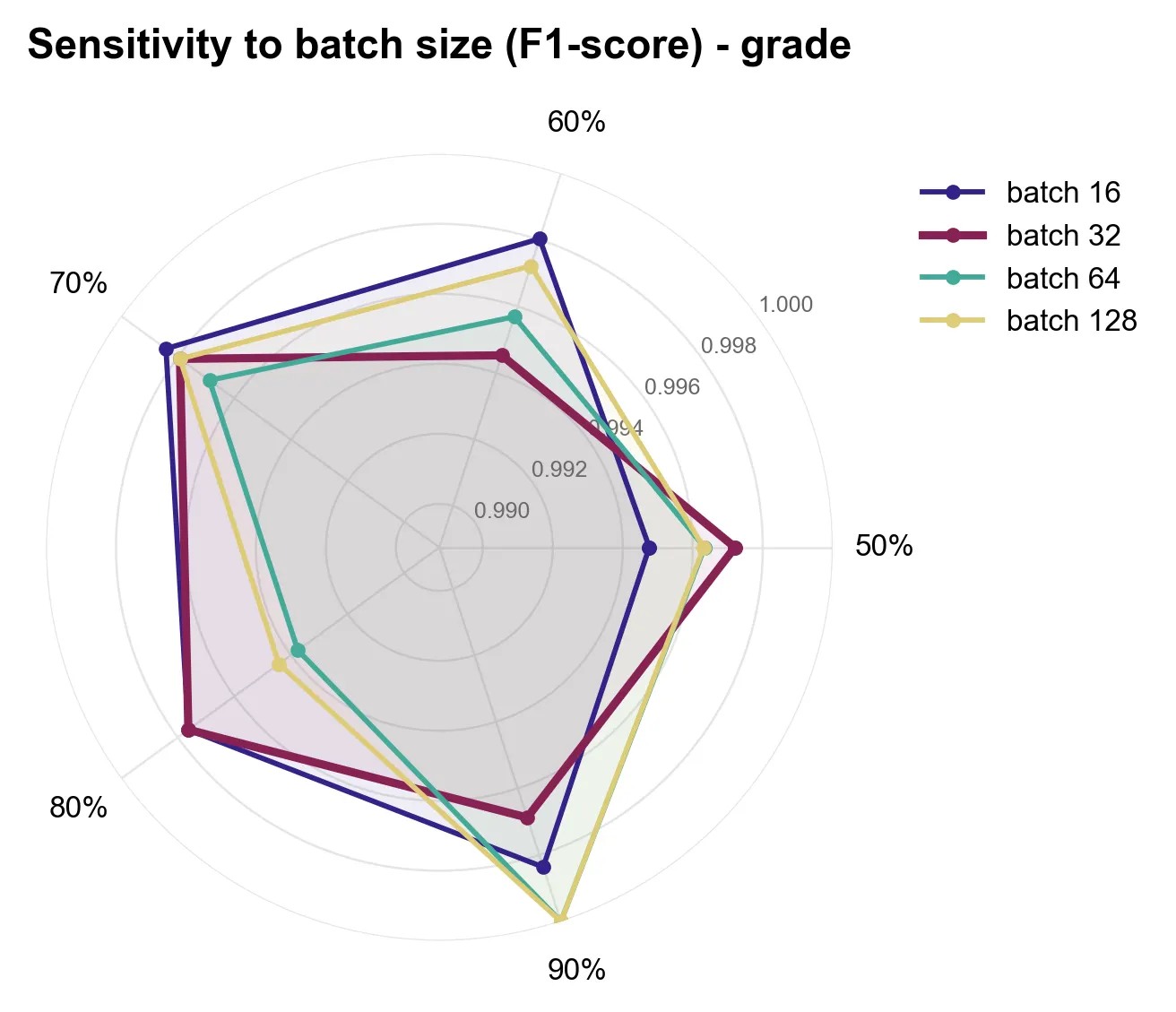
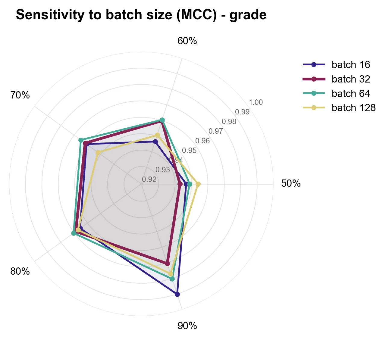
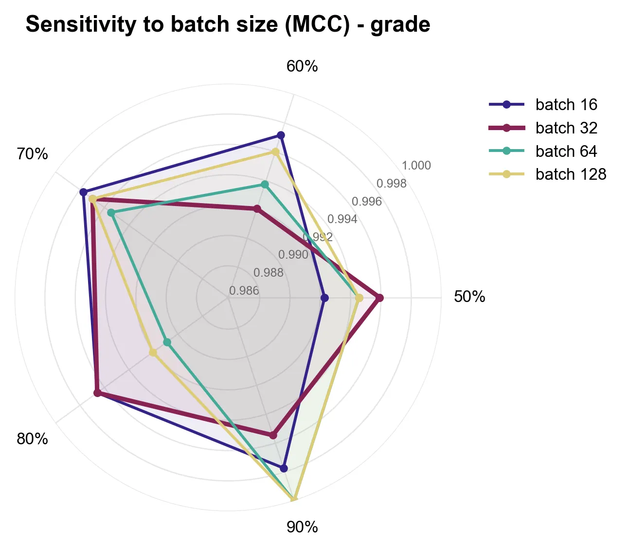
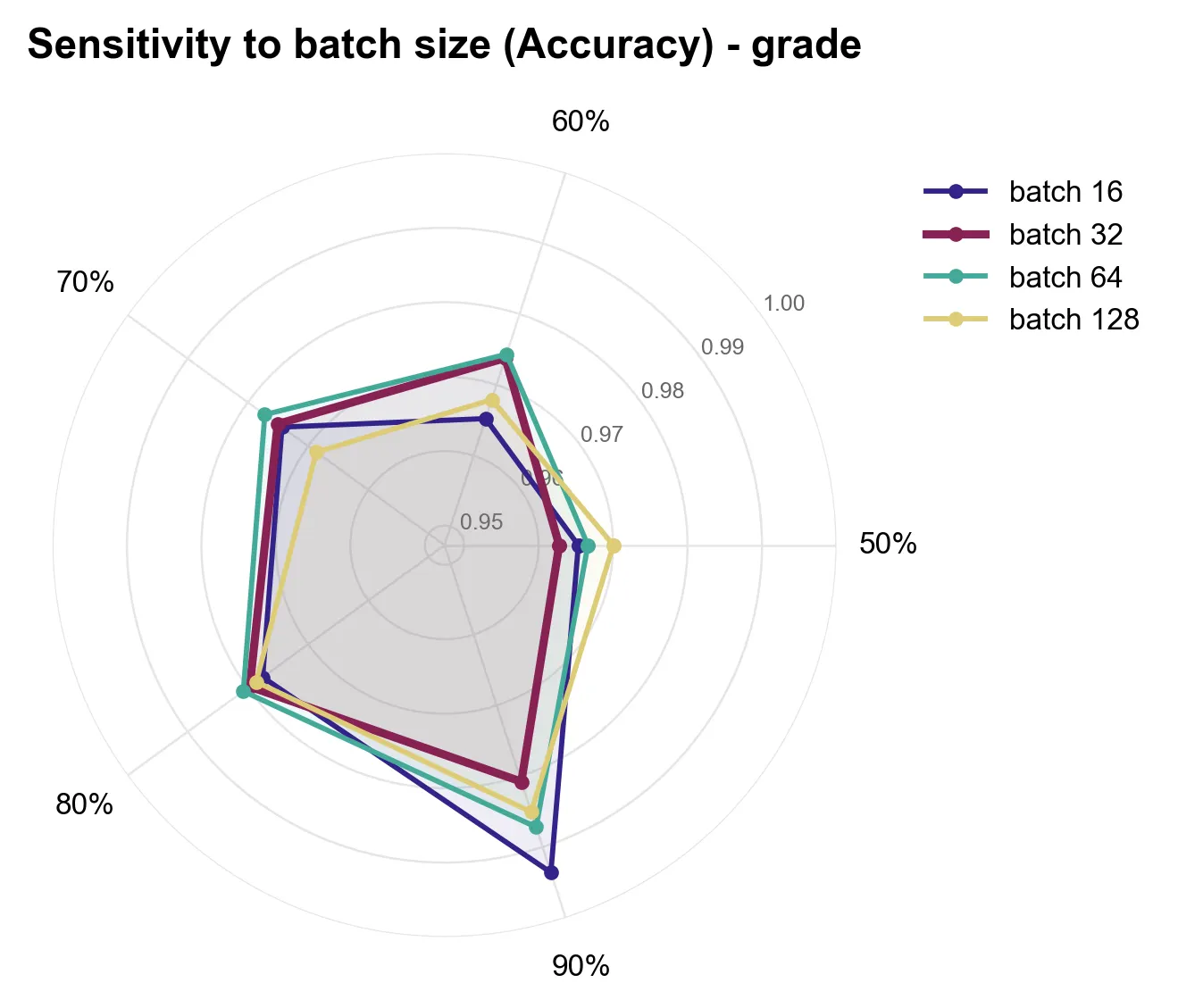
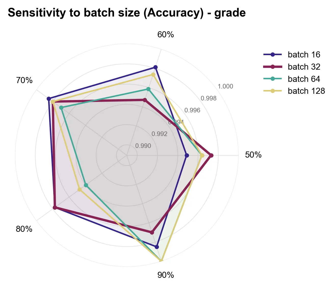
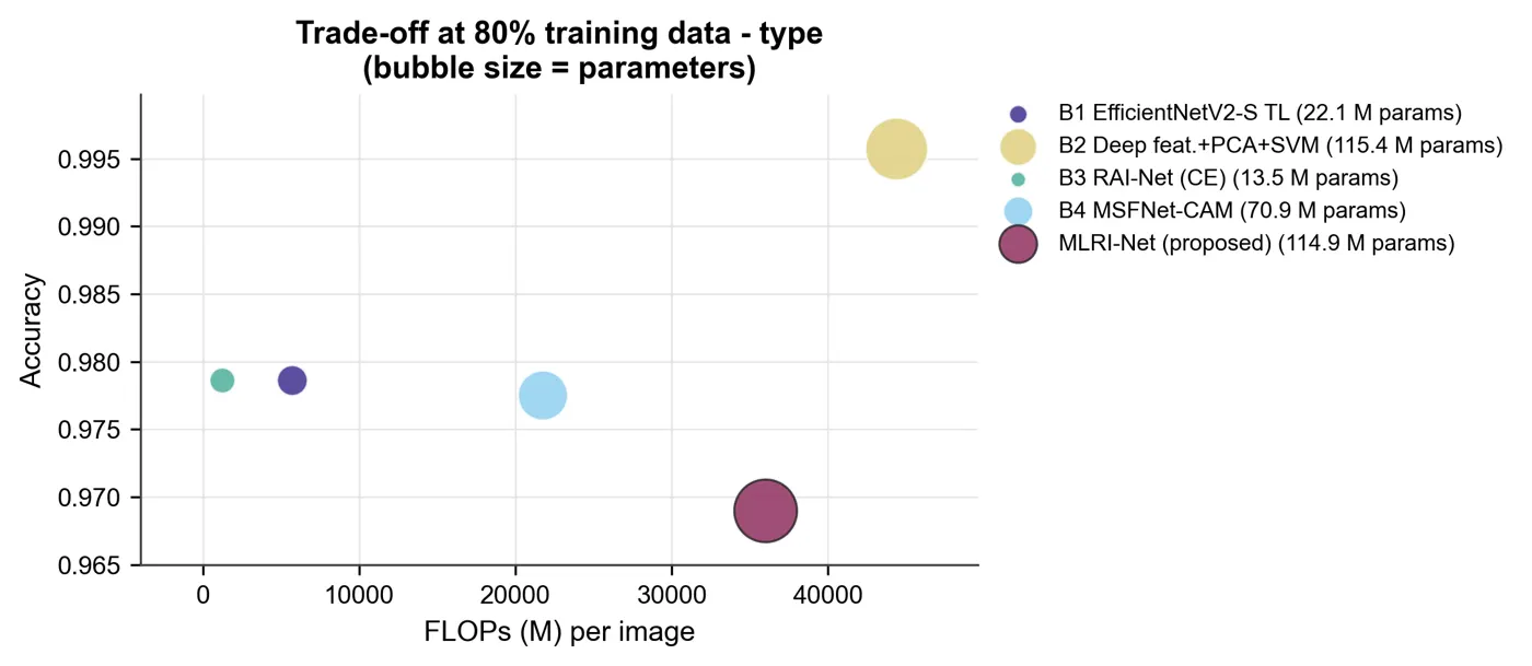
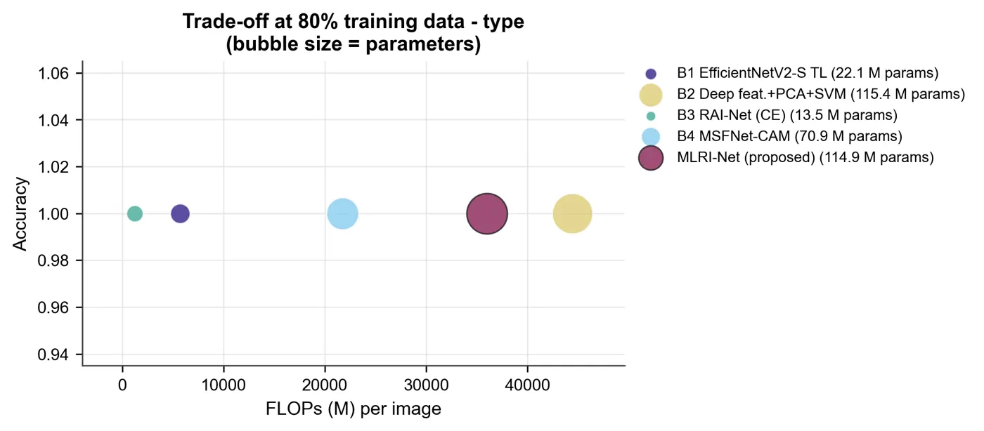
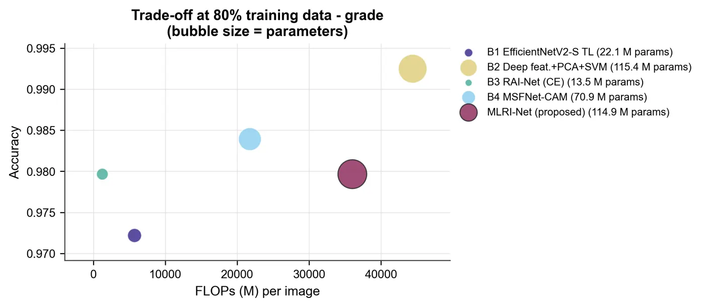
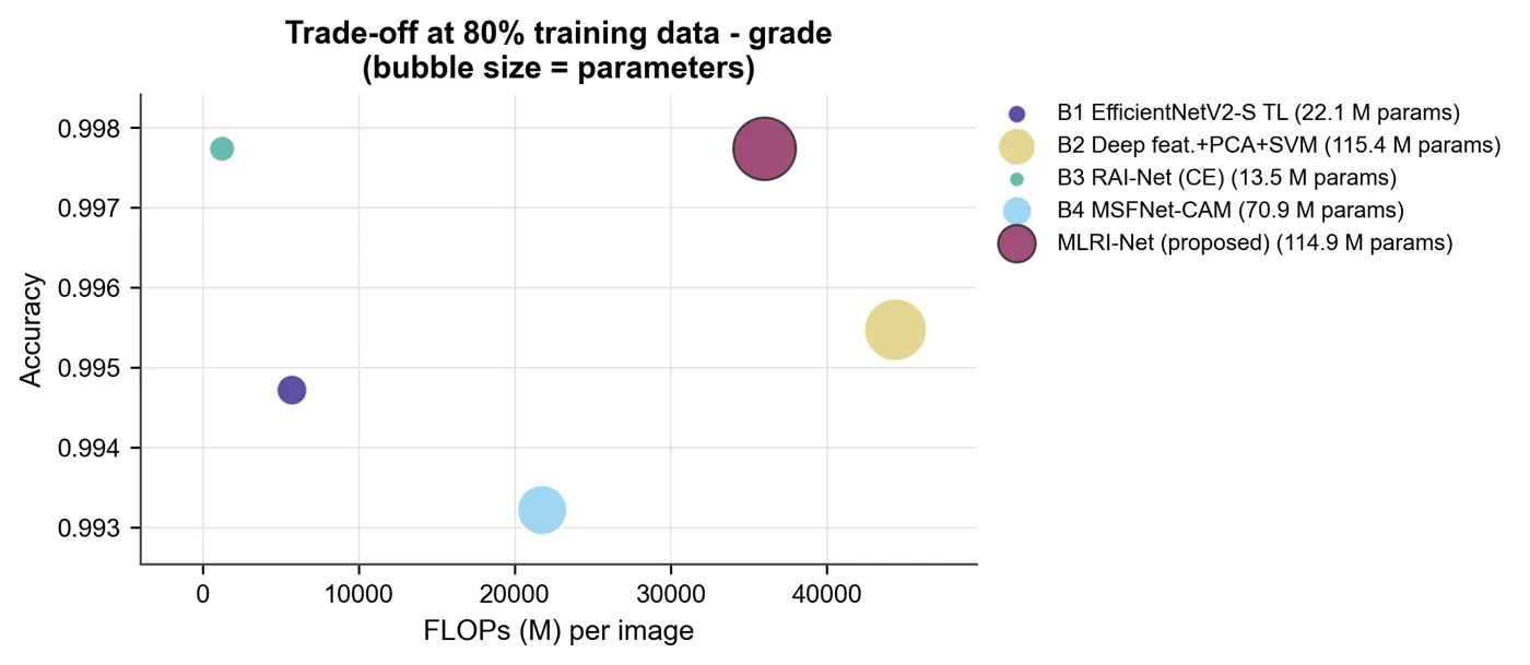
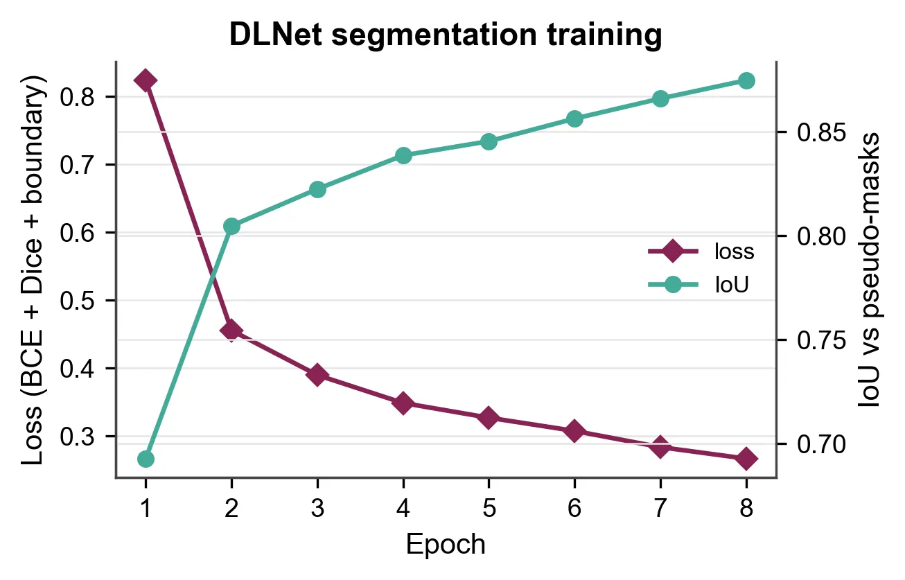
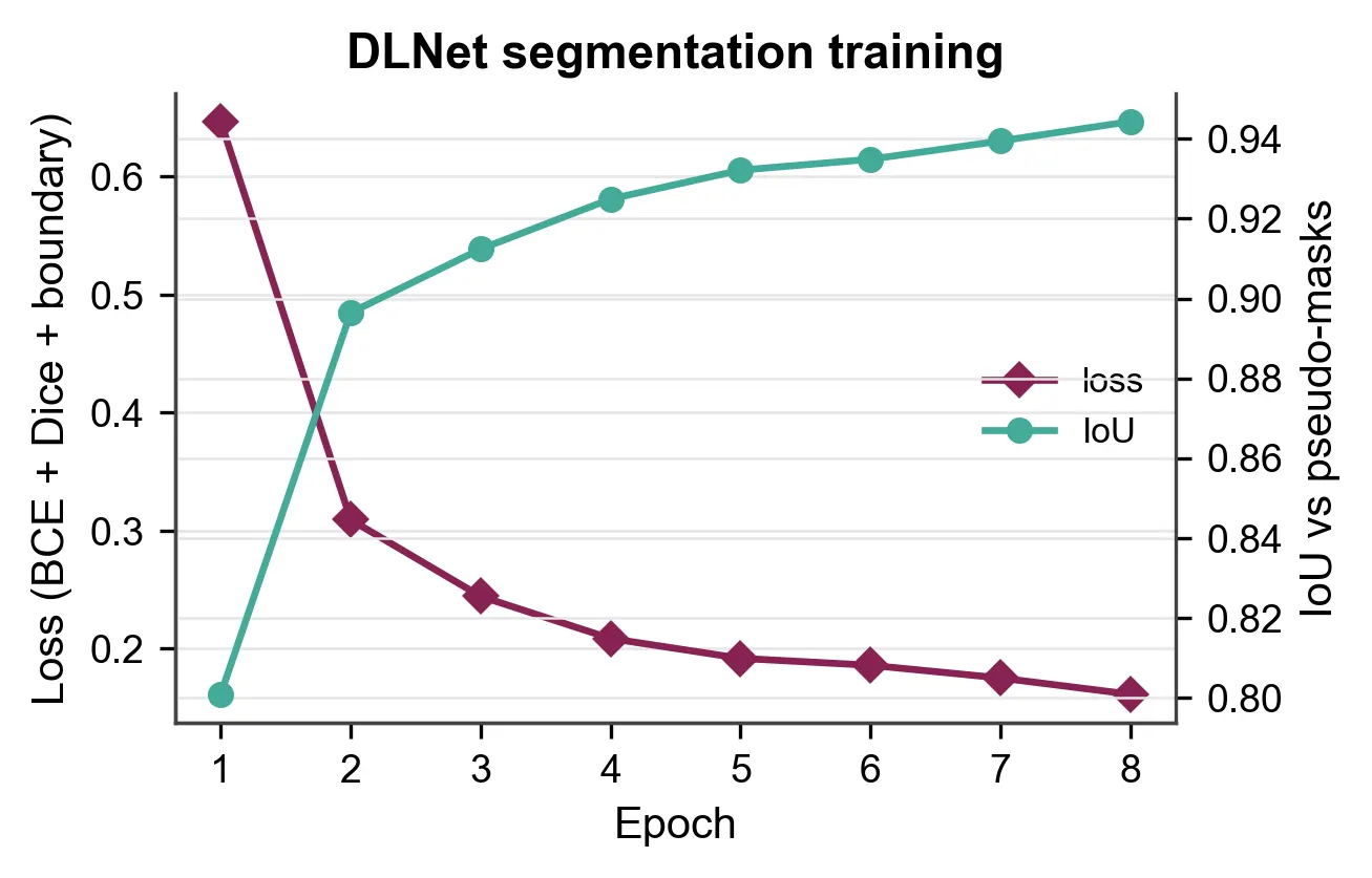
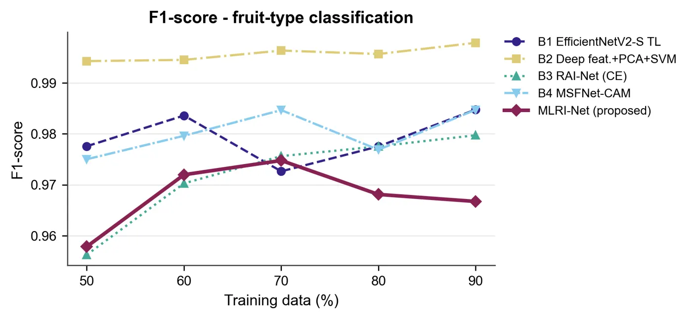
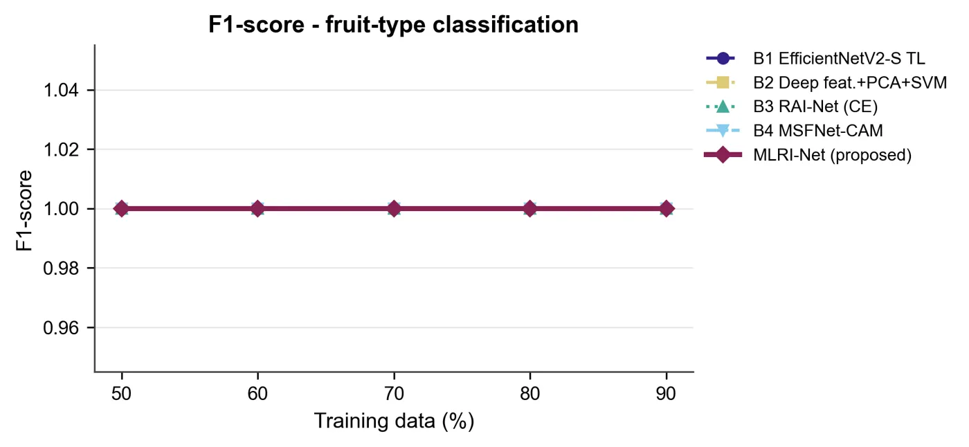
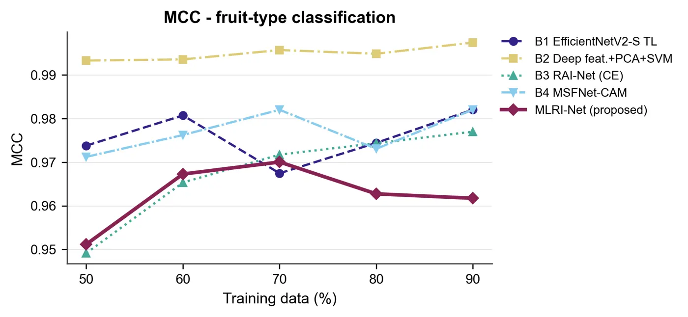
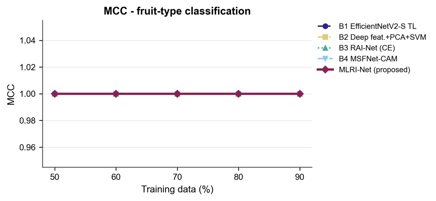
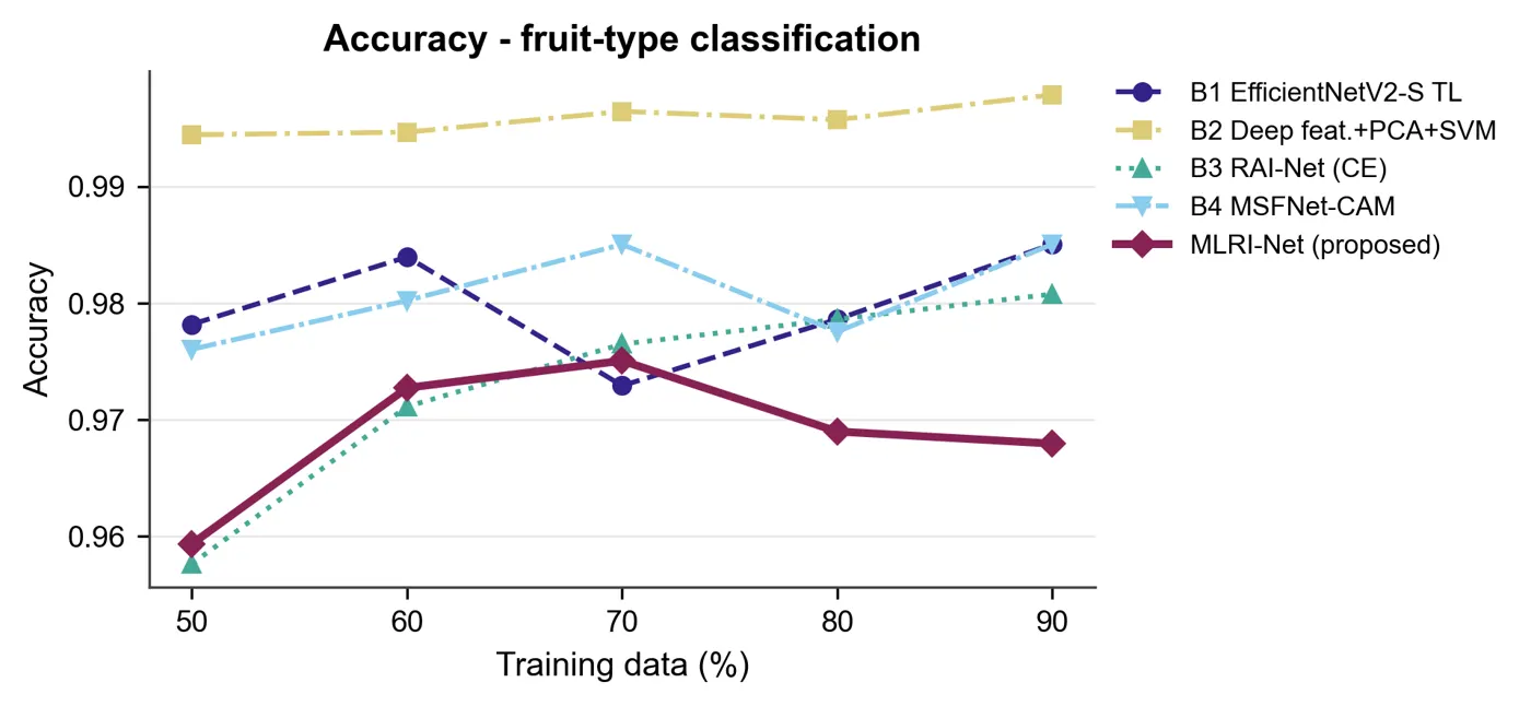
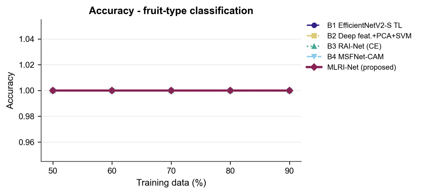
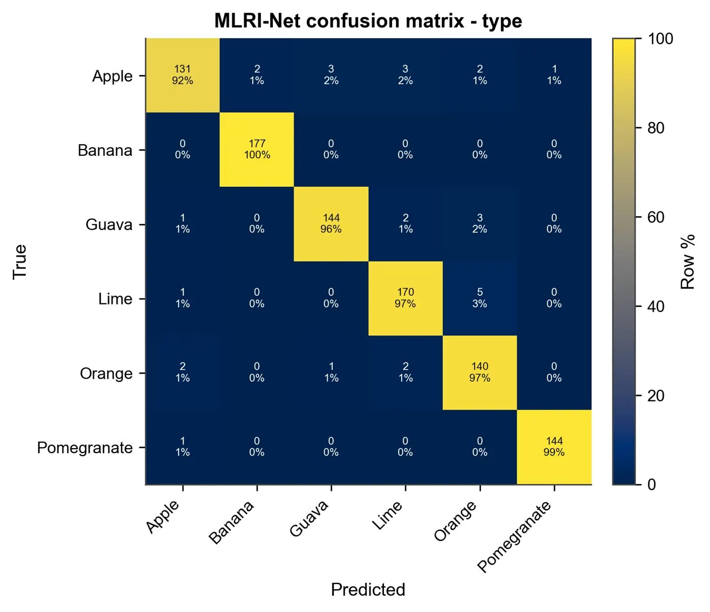
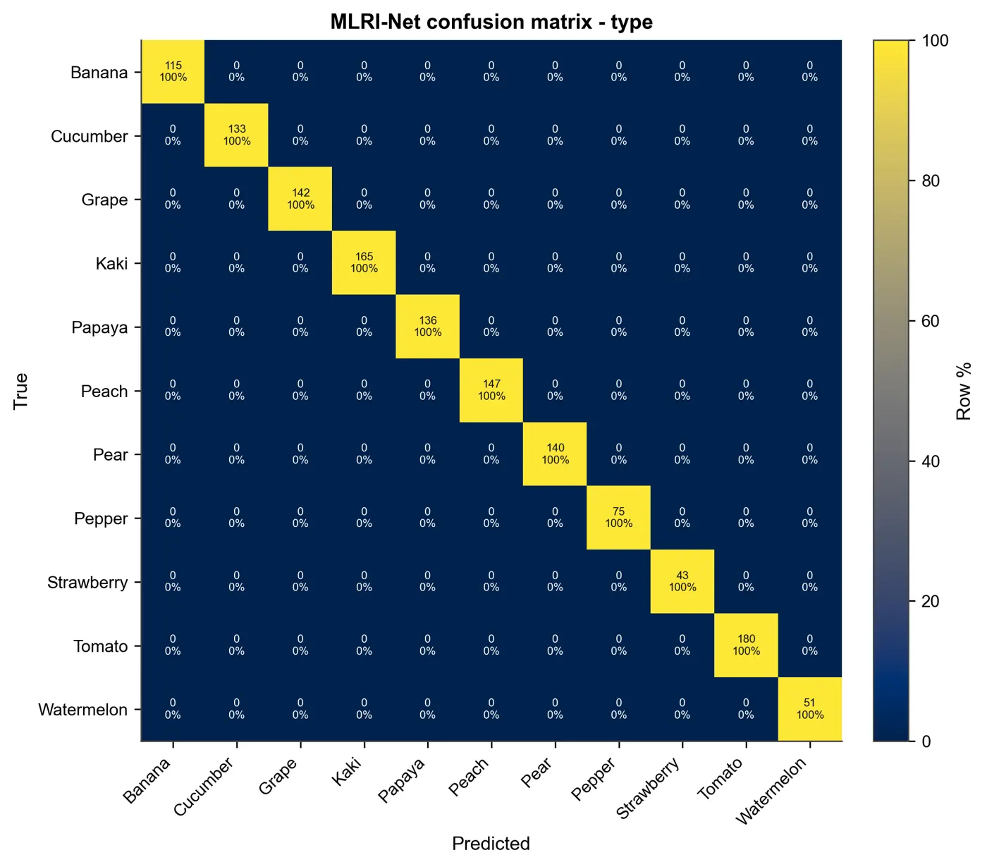
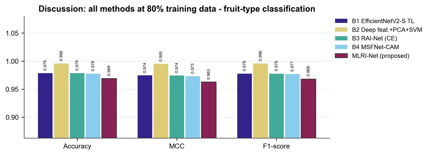
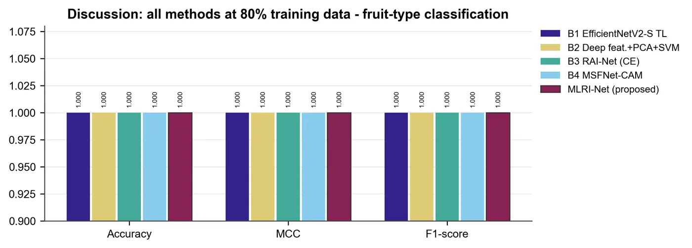
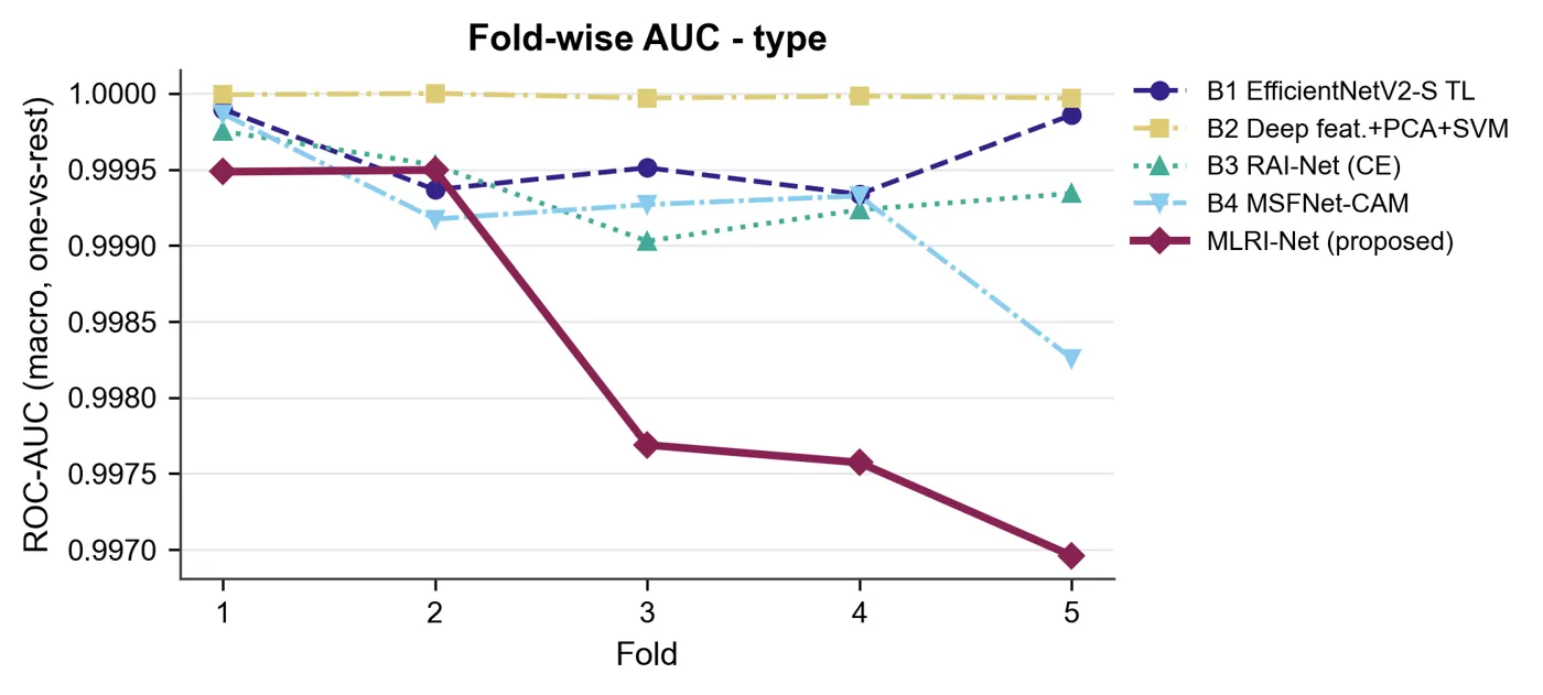
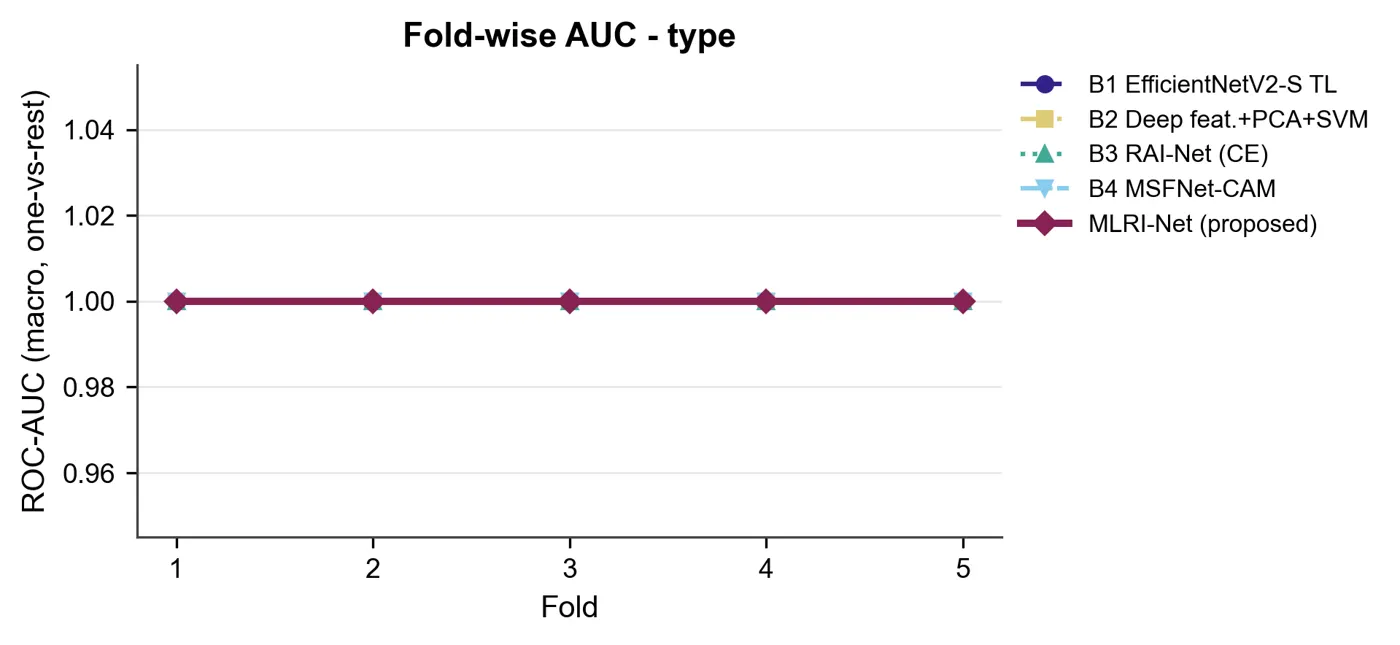
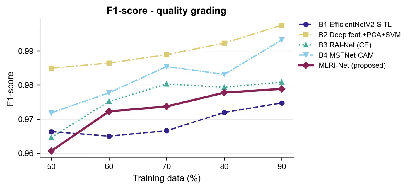
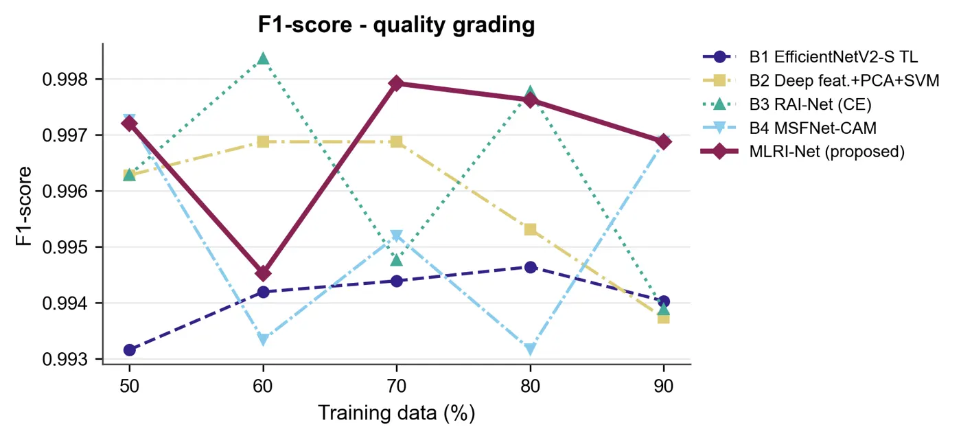
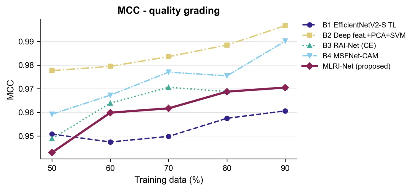
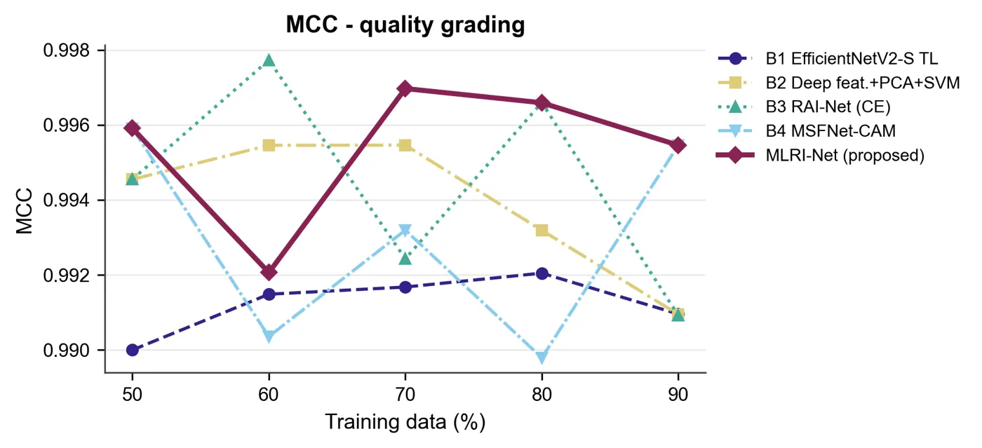
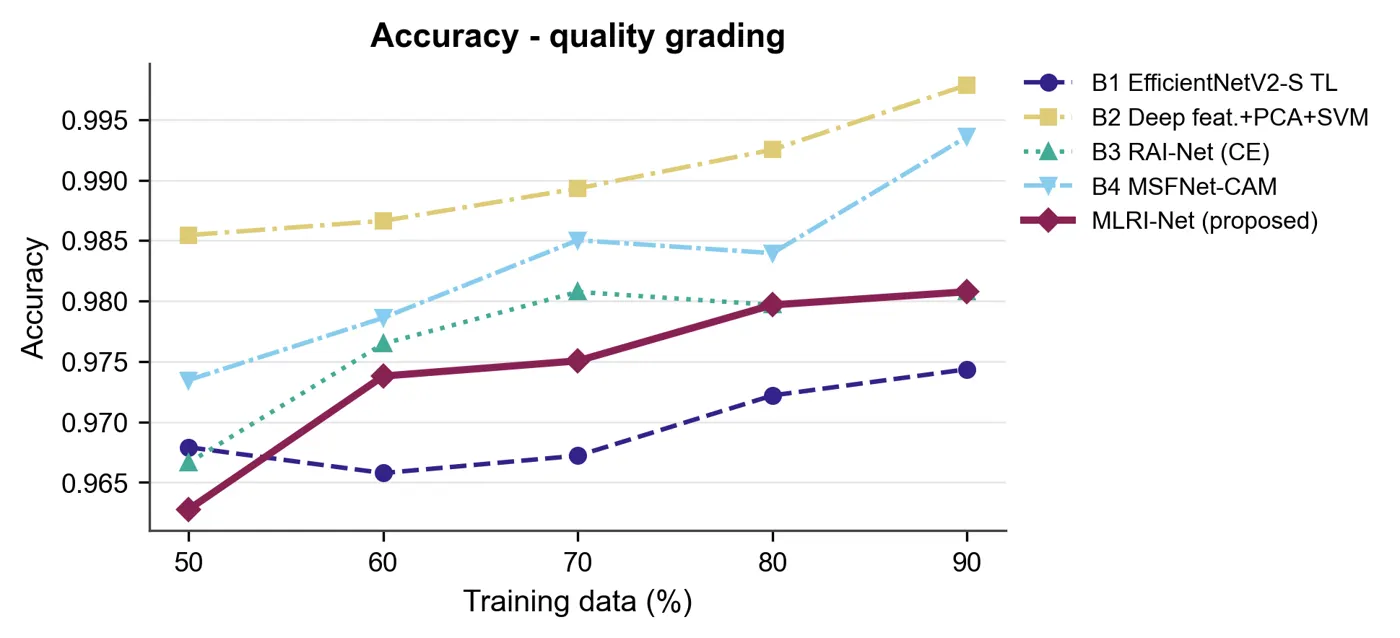
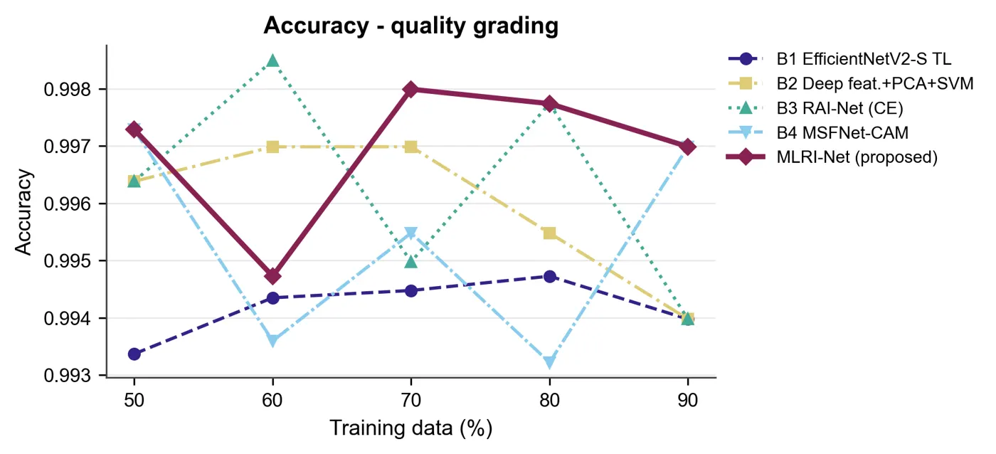
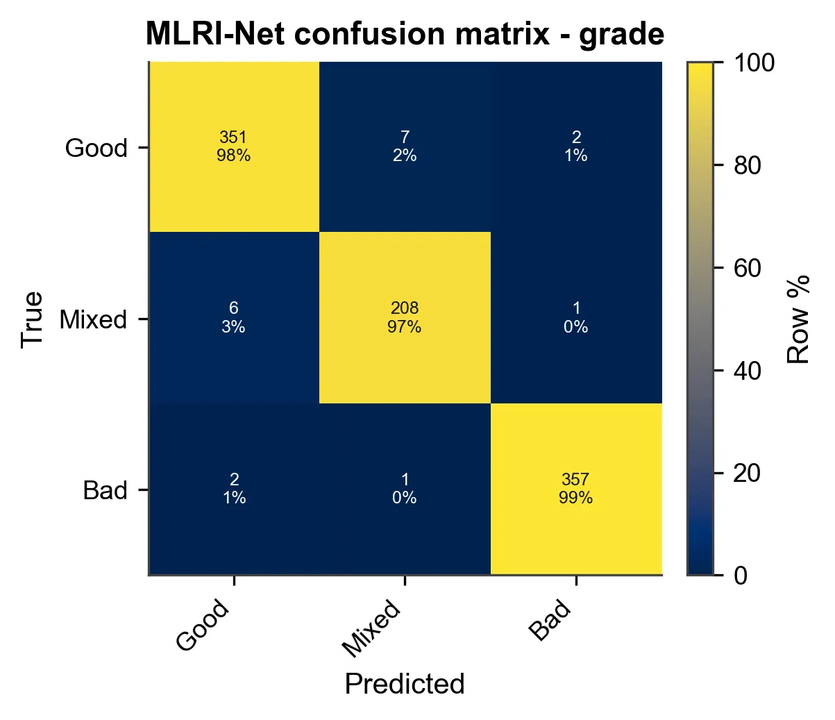
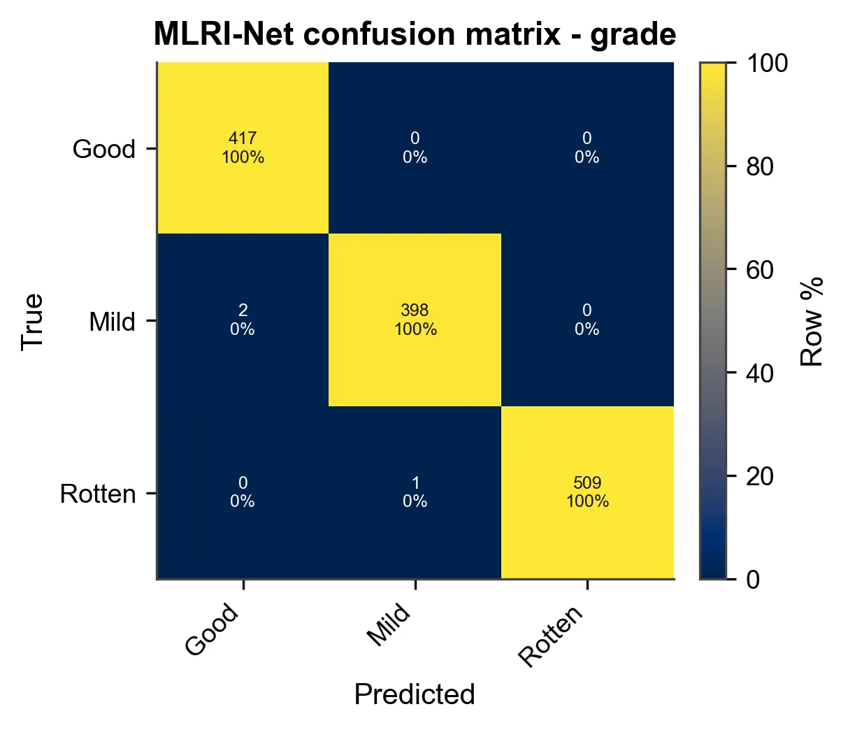
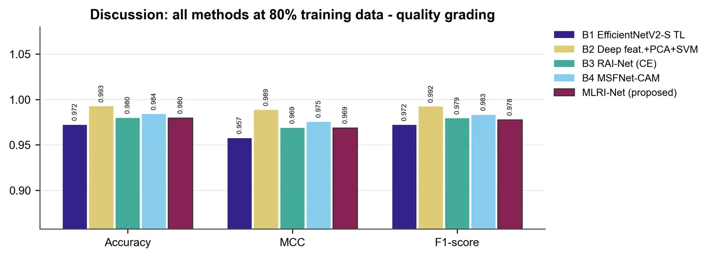
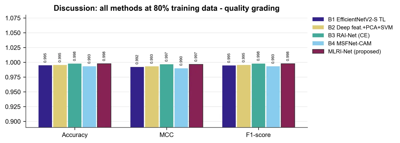
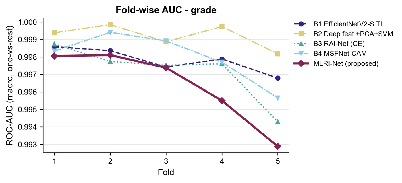
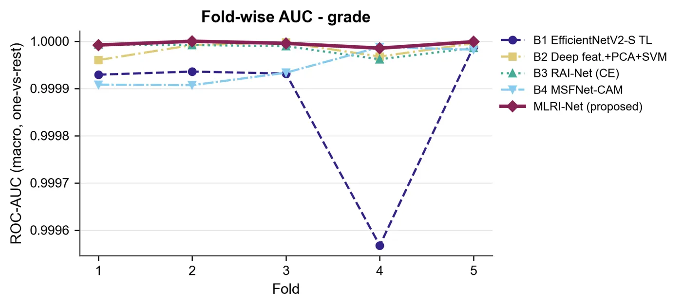
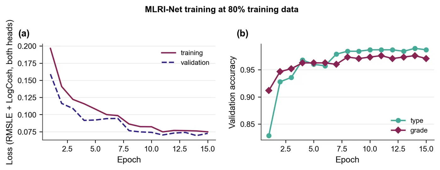
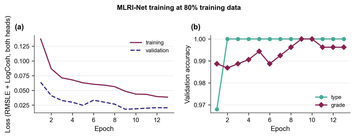
Every graph and diagram the run produced, grouped by purpose. Filter by group and click any graph to enlarge it.
- Delivered
- 85 graphs and diagrams, all shown
- Formats
- PNG, vector PDF and CSV for each
Loading the PDF… 0%
The manuscript as written, before any journal formatting, in a PDF viewer with page jump and zoom.
- Length
- 31 pages, before formatting
- Viewer
- Zoom, page jump, full screen, download
Loading the PDF… 0%
The final paper: the same manuscript typeset in the IEEE two-column layout, with figures placed and references formatted.
- Final paper
- 18 pages, IEEE two-column
- Word (DOCX)
- LaTeX source
Author names in the samples are placeholders.
Loading the PDF… 0%
Everything starts from the concept document, together with the proposal, base papers and datasets in one project folder. Each is read and scored before anything is written.
- Concept PDF, 11 handwritten pages
- Cleveland heart-disease dataset
- Base papers
The concept document is the starting point. Scroll through all 11 pages in the viewer.
"""
ShPCN-Net research control panel (tkinter GUI).

* "Run Full Pipeline & Show Graphs" runs every step for the chosen dataset(s) on a
  background thread and then shows all result graphs in the built-in viewer.
* Every pipeline step can also be run on its own from the left-hand menu.
* Settings: dataset selector (or "All datasets"), DATA_PERCENT (1-100), a toggle that
  draws a new random seed (a new set of results), and a quick smoke-test mode.

Run:  python main.py
"""
import os
import platform
import queue
import subprocess
import sys
import threading
import tkinter as tk
import traceback
from tkinter import messagebox, ttk

from PIL import Image, ImageTk

import full_pipeline_runner as runner
import run_config as cfg
from data_loader import discover_datasets

ALL_DATASETS = "All datasets"
ACCENT = "#D55E00"
INK = "#1B1B1B"
PANEL = "#F6F4F1"


def open_folder(path):
    path.mkdir(parents=True, exist_ok=True)
    if platform.system() == "Windows":
        os.startfile(str(path))
    elif platform.system() == "Darwin":
        subprocess.Popen(["open", str(path)])
    else:
        subprocess.Popen(["xdg-open", str(path)])


class ControlPanel(tk.Tk):
    def __init__(self):
        super().__init__()
        self.title("ShPCN-Net · Heart Disease Detection · Research Control Panel")
        # fit the window to the screen (laptops with 125-150 % scaling report ~1536 x 864)
        width = min(1360, self.winfo_screenwidth() - 40)
        height = min(860, self.winfo_screenheight() - 90)
        self.geometry(f"{width}x{height}+10+10")
        self.minsize(min(1000, width), min(600, height))
        self.configure(bg=PANEL)
        self.messages = queue.Queue()
        self.worker = None
        self.graph_paths = []
        self.preview_image = None
        self.datasets = list(discover_datasets())
        self._build_style()
        self._build_header()
        self._build_body()
        self._drain_job = self.after(150, self._drain_messages)
        self.refresh_gallery()
        if not self.datasets:
            messagebox.showerror("No dataset", "No non-empty code/dataset_*/ folder was found.\n"
                                               "Add the dataset before running the pipeline.")

    # ------------------------------------------------------------------ layout
    def _build_style(self):
        style = ttk.Style(self)
…
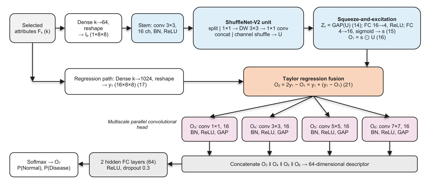
"""
Proposed method - ShPCN-Net (context.docx, Stage 3; concept handwritten diagram p.3):
F_s --(3a embedding)--> I_p --[ShuffleNet-V2 + SE]--> O1
F_s --(regression y1)--+
+--[Taylor fusion O2 = 2*y1 - O1]--> O2 --[PCNN 1/3/5/7]--> O3..O6
O7 = softmax( fc( O3 || O4 || O5 || O6 ) ) -> Disease / Normal
"""
import torch
from torch import nn
from network_building_blocks import (FeatureToMapEmbedding, HiddenDenseStack, ParallelMultiscaleConv,
ShuffleNetSEBranch, TaylorRegressionFusion)
from torch_training_loop import TorchTabularClassifier
class ShPCNNetModule(nn.Module):
def __init__(self, n_features, s):
super().__init__()
c, m = s["channels"], s["map_size"]
self.embedding = FeatureToMapEmbedding(n_features, m) # 3a
self.shufflenet_branch = ShuffleNetSEBranch(c, s["se_reduction"]) # 3b
self.taylor_fusion = TaylorRegressionFusion(n_features, c, m) # 3c
self.pcnn = ParallelMultiscaleConv(c, s["pcnn_filters"], s["pcnn_kernel_sizes"]) # 3d
self.head = HiddenDenseStack(s["pcnn_filters"] * len(s["pcnn_kernel_sizes"]),
s["hidden_neurons"], s["hidden_layers"], s["dropout_rate"],
s["activation"])
def forward(self, features, return_intermediates=False):
i_p = self.embedding(features)
o1, se_weights, unit_map = self.shufflenet_branch(i_p)
o2, y1 = self.taylor_fusion(features, o1)
pooled, branch_maps = self.pcnn(o2)
logits = self.head(pooled)
if not return_intermediates:
return logits
return logits, {
"I_p": i_p, "shufflenet_unit_map": unit_map, "se_weights": se_weights,
"O1": o1, "y1": y1, "O2": o2,
"O3": branch_maps[0], "O4": branch_maps[1], "O5": branch_maps[2], "O6": branch_maps[3],
"O7": torch.softmax(logits, dim=1),
}
class ShPCNNetClassifier(TorchTabularClassifier):
display_name = "ShPCN-Net (proposed)"
def build_module(self, n_features):
return ShPCNNetModule(n_features, self.settings)
def trace_intermediates(self, X):
"""Every intermediate tensor (as numpy) for visualisation of one or more samples."""
self.module.eval()
with torch.no_grad():
_, inter = self.module(torch.as_tensor(X, dtype=torch.float32), return_intermediates=True)
return {k: v.numpy() for k, v in inter.items()}
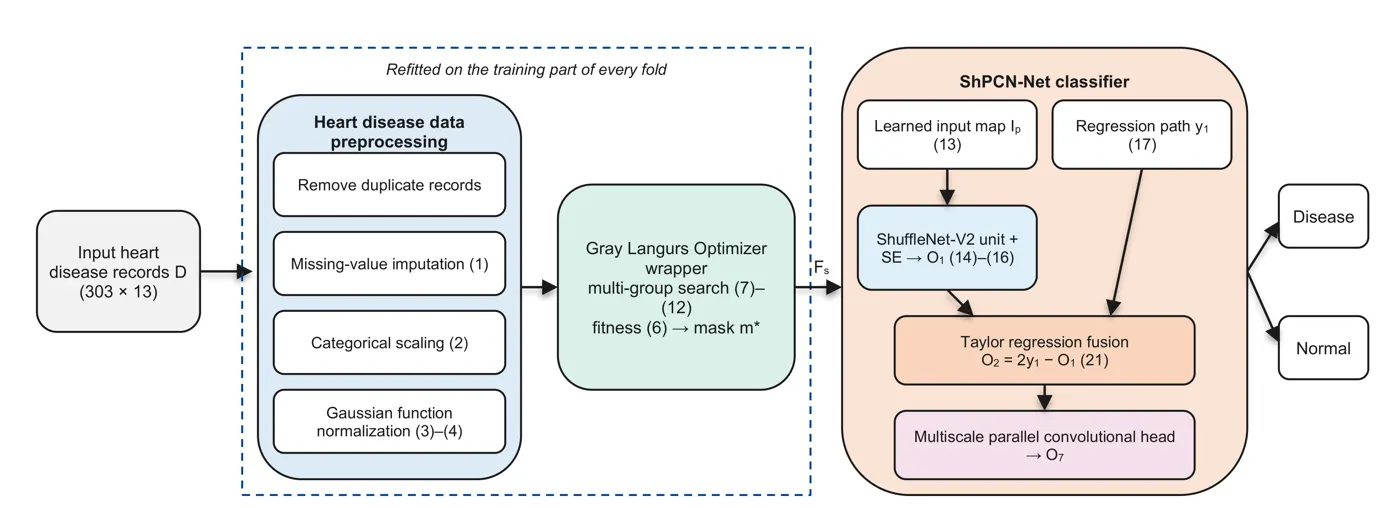
"""
Stage 2 - feature selection with the Gray Langurs Optimizer (GLO)  (N_d -> F_s).

Source: Barshandeh et al., "Gray langurs optimizer: a multi-group bio-inspired
optimization algorithm" (Artificial Intelligence Review, 2026). The paper is not
in basepapers/, so the equations below follow its published description (three
group types: one-male, multi-male and all-male groups; social hierarchy;
migration between groups after alpha death / mate finding / puberty; arbitrary
movement inside the territory). The exact coefficients are our documented
interpretation - see context.docx "Open questions".

Notation (per langur i, dimension d, iteration t of T):
  a      = a_start - (a_start - a_end) * t / (T - 1)       control parameter, 2 -> 0
  r1,r2,r3 ~ U(0,1)
  One-male group  (follow the single alpha A_g):
      X_new = A_g - a * (2*r1 - 1) * |r2 * A_g - X_i|
  Multi-male group (follow the mean M_g of the top-3 males + global best G):
      X_new = M_g - a * (2*r1 - 1) * |r2 * M_g - X_i| + r3 * (1 - a/a_start) * (G - X_i)
  All-male group  (bachelors roam: random partner X_j + pull to G for mate finding):
      X_new = X_i + a * (2*r1 - 1) * (X_j - X_i) + r2 * (1 - a/a_start) * (G - X_i)
  Territory movement (probability p_rand):
      X_new = X_i + a * N(0, 0.1 * (ub - lb))
  Greedy replacement: X_i <- X_new only if fitness improves.
  Alpha death: if a group's best fitness has not improved for L iterations, its
      worst member is re-born near the global best (puberty / new male joins).
  Migration: every M iterations the worst member of group g swaps with a random
      member of group g+1 (langurs move between groups).
  Boundaries: positions are clipped to [lb, ub].

Solution encoding (context.docx 3.3.1): position vector in [0,1]^N, feature d is
selected when X_d > 0.5 -> equivalent to the list of selected feature indices.
Fitness (Eq. 24): Fitness = alpha*(1 - Accuracy) + (1 - alpha) * R / K  (minimised),
Accuracy from an RBF-SVM wrapper with stratified inner CV on the training data only.
"""
import numpy as np
from sklearn.model_selection import StratifiedKFold, cross_val_score
from sklearn.svm import SVC

import run_config as cfg

GROUP_TYPES = ("one_male", "multi_male", "all_male")


def position_to_mask(position, threshold):
    """Continuous langur position -> boolean feature mask (at least one feature)."""
    mask = position > threshold
    if not mask.any():
        mask[int(np.argmax(position))] = True
    return mask


class FeatureSubsetFitness:
    """Eq. (24) wrapper fitness with a cache (identical masks are scored once)."""

    def __init__(self, X, y, alpha, cv_folds, svm_c, seed, threshold):
        self.X, self.y = X, y
        self.alpha, self.threshold = alpha, threshold
        n_splits = int(max(2, min(cv_folds, np.bincount(y).min())))
        self.cv = StratifiedKFold(n_splits=n_splits, shuffle=True, random_state=seed)
        self.svm_c = svm_c
        self.cache = {}

    def accuracy_of(self, mask):
        key = tuple(np.flatnonzero(mask))
        if key not in self.cache:
            model = SVC(C=self.svm_c, kernel="rbf", gamma="scale")
            self.cache[key] = float(cross_val_score(model, self.X[:, mask], self.y, cv=self.cv).mean())
        return self.cache[key]

    def __call__(self, position):
…
"""
Reusable PyTorch blocks for ShPCN-Net and the ablation baselines (context.docx, Stage 3).
FeatureToMapEmbedding 3a: k selected features -> learned 1 x 8 x 8 map I_p
ShuffleNetV2Unit 3b: channel split, 1x1 conv, 3x3 depthwise conv, 1x1 conv,
concatenation, channel shuffle
SqueezeExcitation 3b: Eq. 8-10 Z_c = 1/(H*W) sum_i sum_j I_p
s = sigma(W2 * delta(W1 * Z_c))
O1 = s * I_p
TaylorRegressionFusion 3c: y1 = sum F_i * w_i (learned map to the shape of O1)
O2 = 2*y1 - O1 (first-order Taylor rule, k = 1)
ParallelMultiscaleConv 3d: O3..O6 = f_conv1..4(O2) with 1/3/5/7 kernels
HiddenDenseStack FC hidden layers (depth = "hidden layers" setting)
"""
import torch
from torch import nn
def make_activation(name):
return {"relu": nn.ReLU(), "gelu": nn.GELU(), "elu": nn.ELU(), "tanh": nn.Tanh()}.get(name, nn.ReLU())
class FeatureToMapEmbedding(nn.Module):
"""Dense k -> map_size^2, reshaped to (B, 1, H, W). This is the network input I_p."""
def __init__(self, n_features, map_size):
super().__init__()
self.map_size = map_size
self.linear = nn.Linear(n_features, map_size * map_size)
def forward(self, x):
return self.linear(x).view(-1, 1, self.map_size, self.map_size)
def channel_shuffle(x, groups):
b, c, h, w = x.shape
return x.view(b, groups, c // groups, h, w).transpose(1, 2).contiguous().view(b, c, h, w)
class ShuffleNetV2Unit(nn.Module):
"""Stride-1 ShuffleNet-V2 basic unit (Ma et al., 2018)."""
def __init__(self, channels):
super().__init__()
half = channels // 2
self.branch = nn.Sequential(
nn.Conv2d(half, half, 1, bias=False), nn.BatchNorm2d(half), nn.ReLU(inplace=True),
nn.Conv2d(half, half, 3, padding=1, groups=half, bias=False), nn.BatchNorm2d(half),
nn.Conv2d(half, half, 1, bias=False), nn.BatchNorm2d(half), nn.ReLU(inplace=True),
)
def forward(self, x):
left, right = x.chunk(2, dim=1) # channel split
out = torch.cat([left, self.branch(right)], dim=1) # concatenation
return channel_shuffle(out, 2) # channel shuffle
class SqueezeExcitation(nn.Module):
"""Eq. 8-10. Returns (O1, s) so the attention weights can be visualised."""
def __init__(self, channels, reduction):
super().__init__()
hidden = max(channels // reduction, 2)
self.w1 = nn.Linear(channels, hidden) # W1
self.w2 = nn.Linear(hidden, channels) # W2
self.delta = nn.ReLU() # delta
self.sigma = nn.Sigmoid() # sigma
def forward(self, i_p):
z_c = i_p.mean(dim=(2, 3)) # Eq. 8: global average pooling
…EasySeer writes the project as separate Python files with a main program. Open any file, read it, and ask the chat what it does.
- In the project
- 47 Python files, plus requirements and a readme
- Shown
- The first lines of four real files
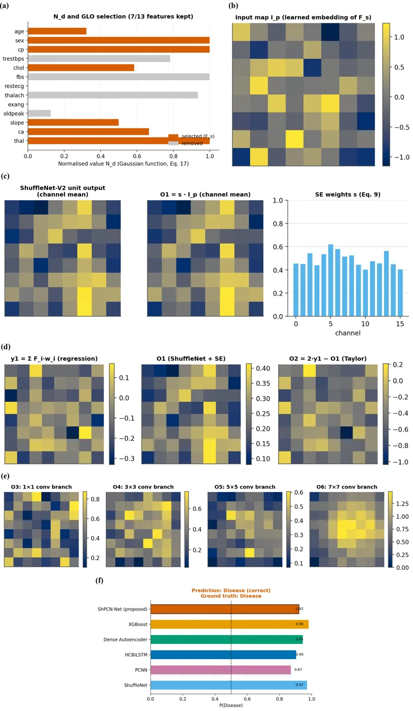
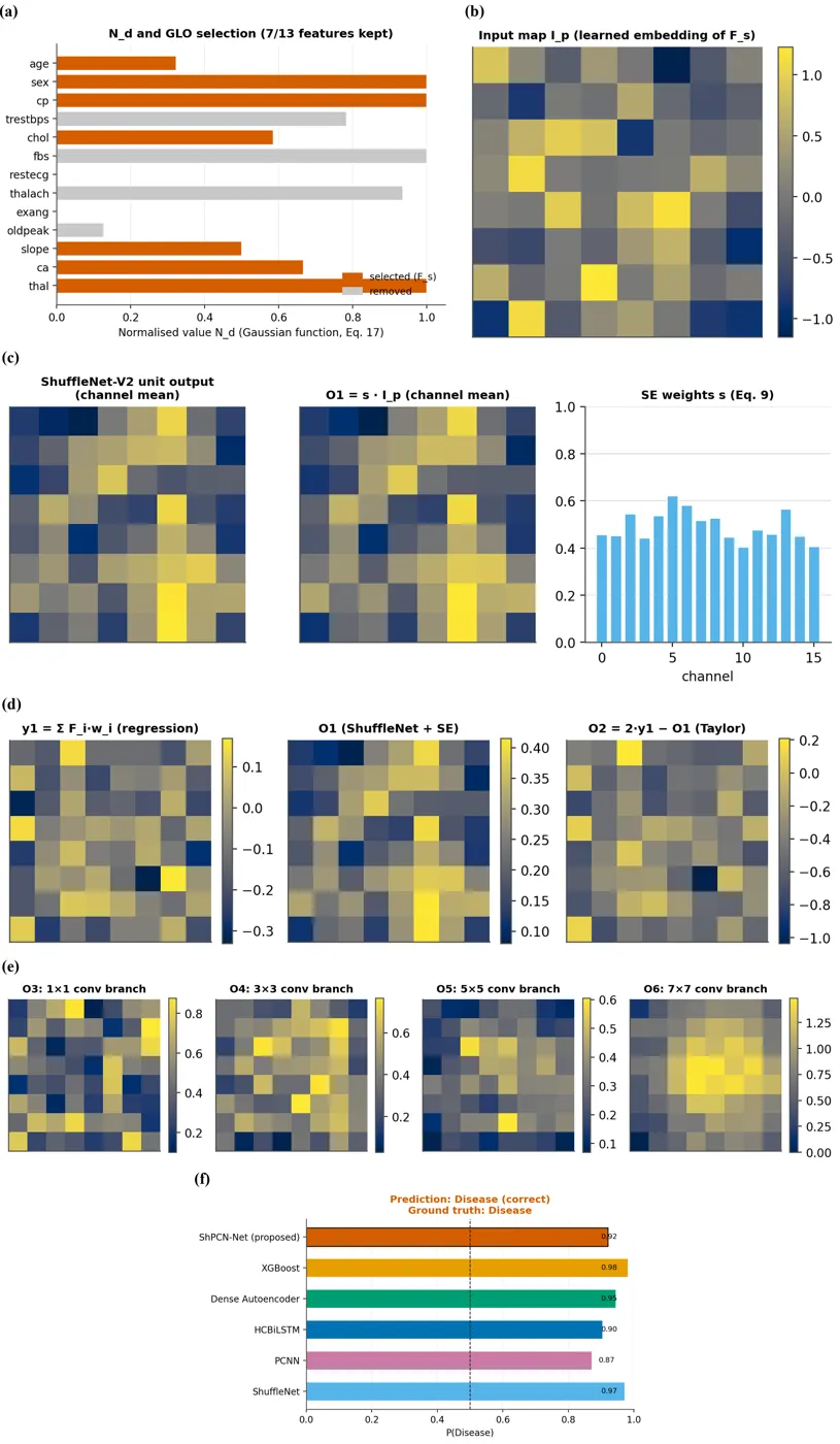
dataset: dataset_cleveland
sample_id: 21 (test sample of fold 1)
selected features (GLO): sex, cp, trestbps, thalach, slope, ca, thal
ShPCN-Net P(Disease) = 0.0324
predicted label: 0 (Normal)
ground truth   : 0 (Normal)

other methods P(Disease):
  ShuffleNet: 0.1355
  PCNN: 0.1273
  HCBiLSTM: 0.0838
  Dense Autoencoder: 0.0315
XGBoost: 0.0080The code runs on your own computer. Every file, log and result is saved to the project folder, so nothing is hidden.
- Records
- 303
- Validation
- 10-fold cross-validation
The text file under the picture is the saved output for that record.
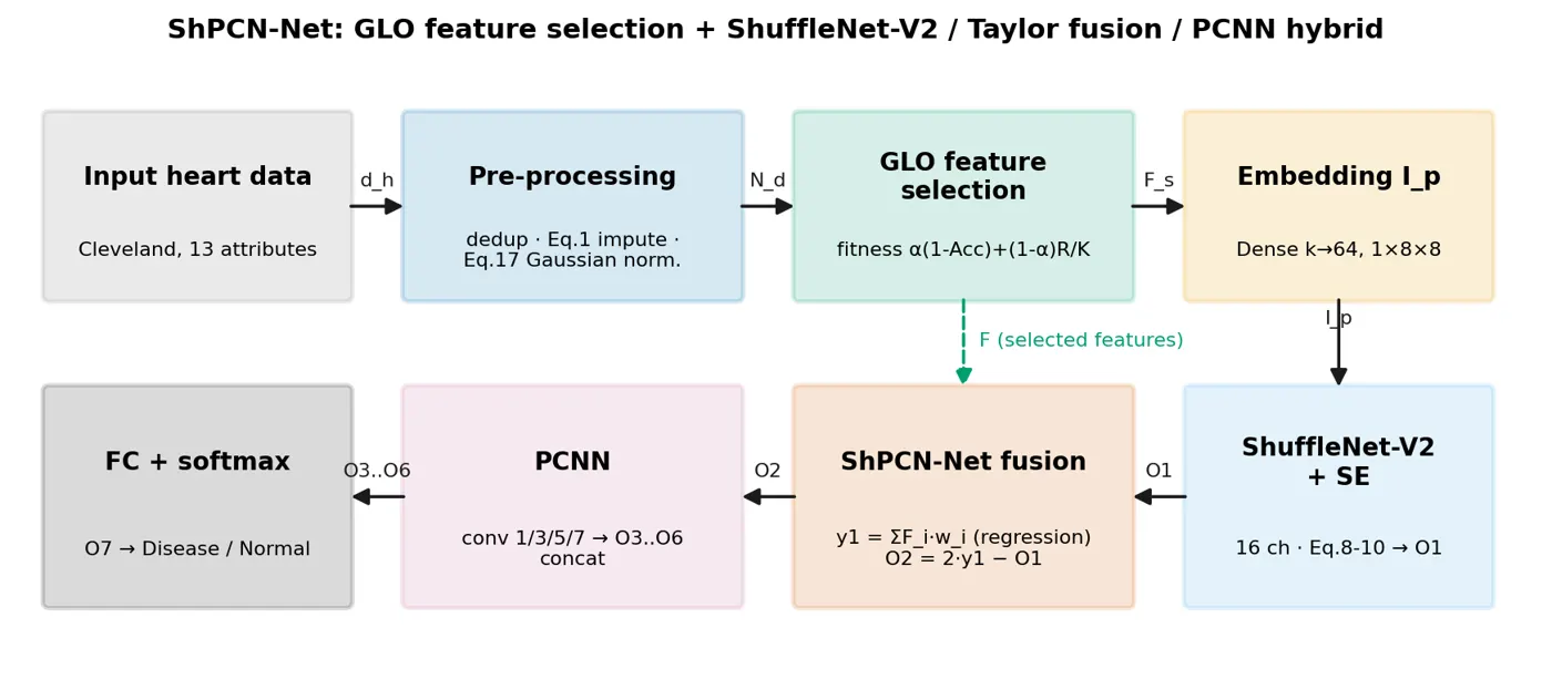
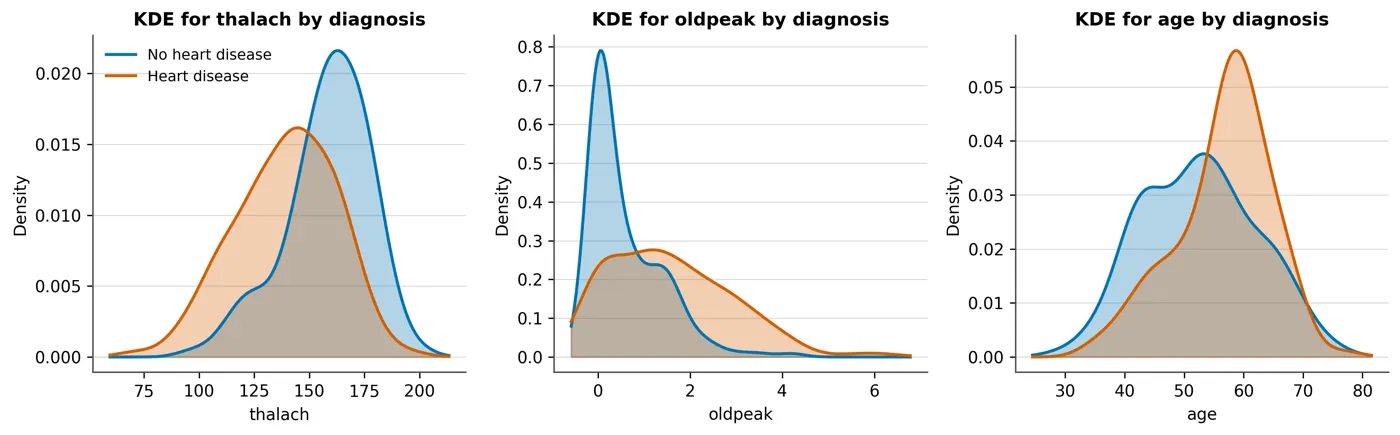
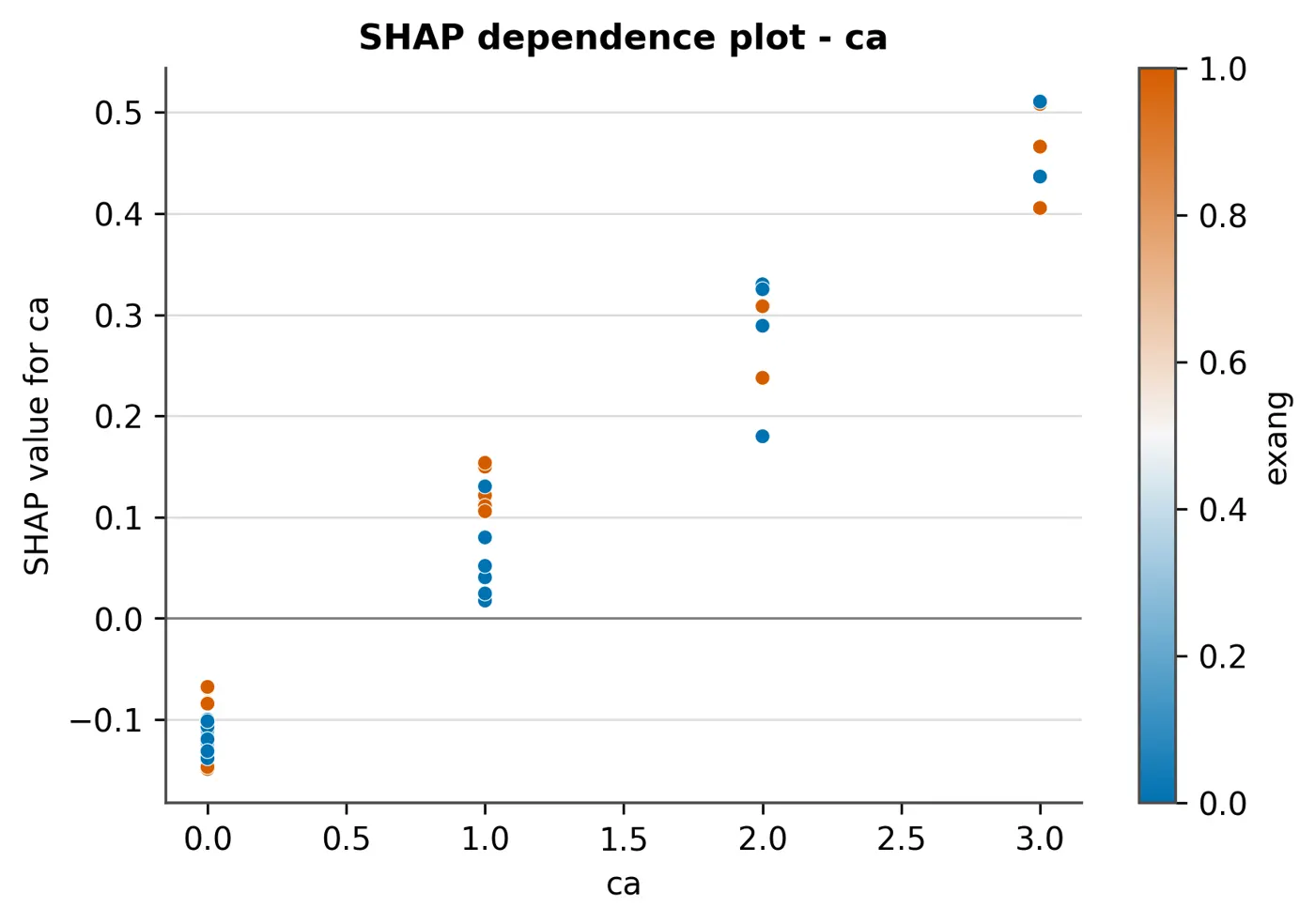
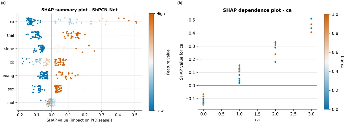
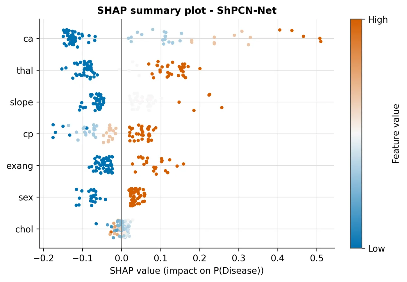
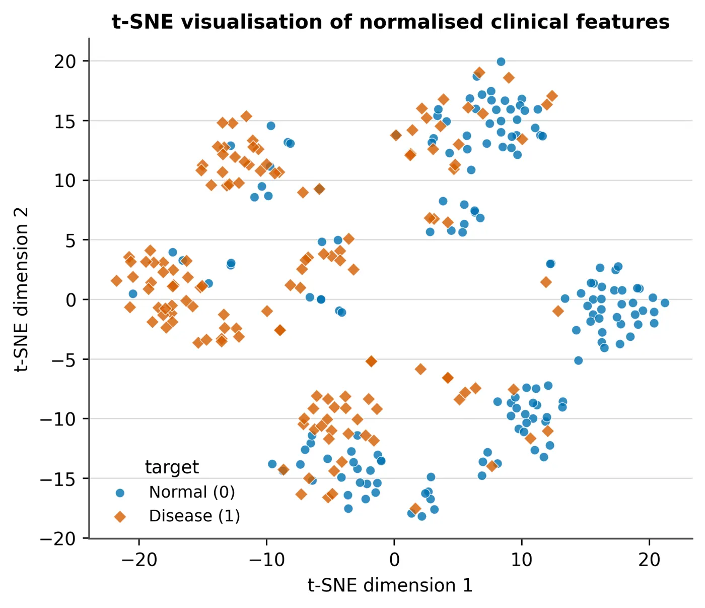
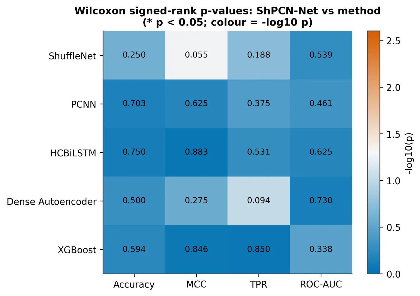
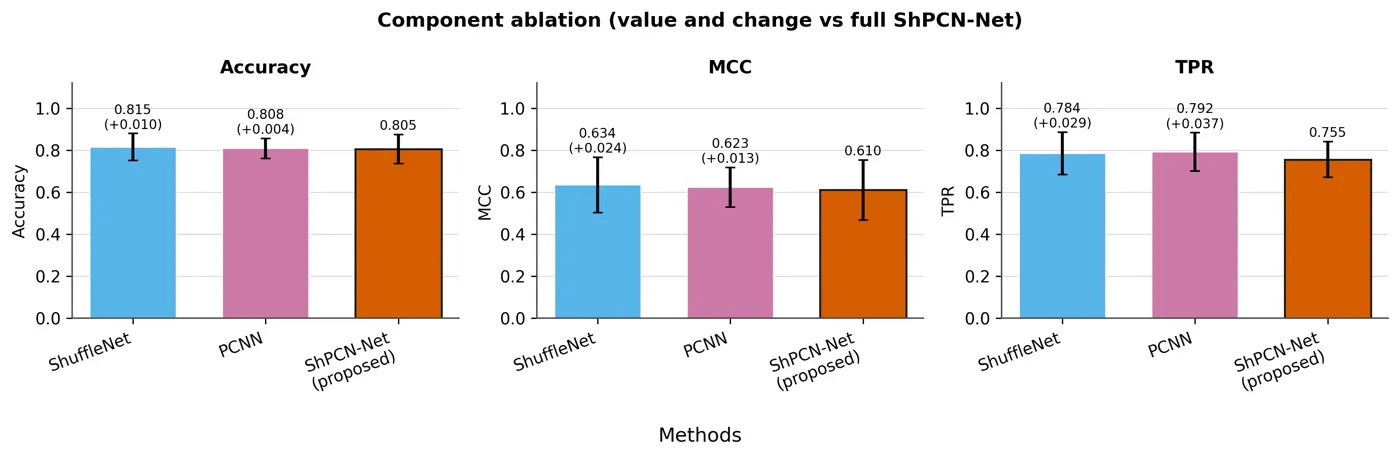
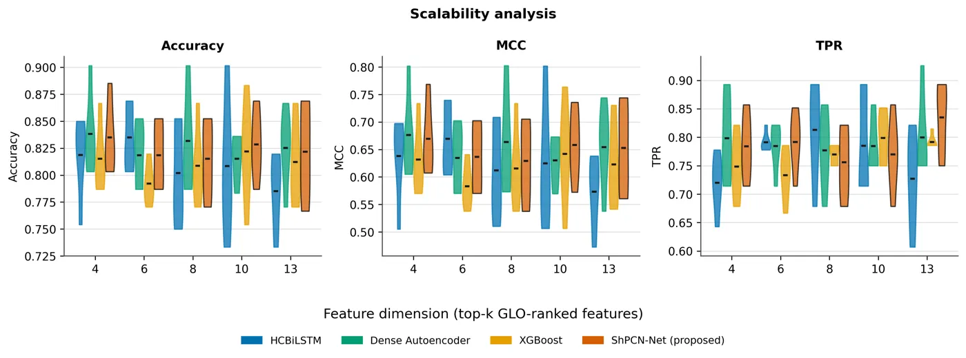
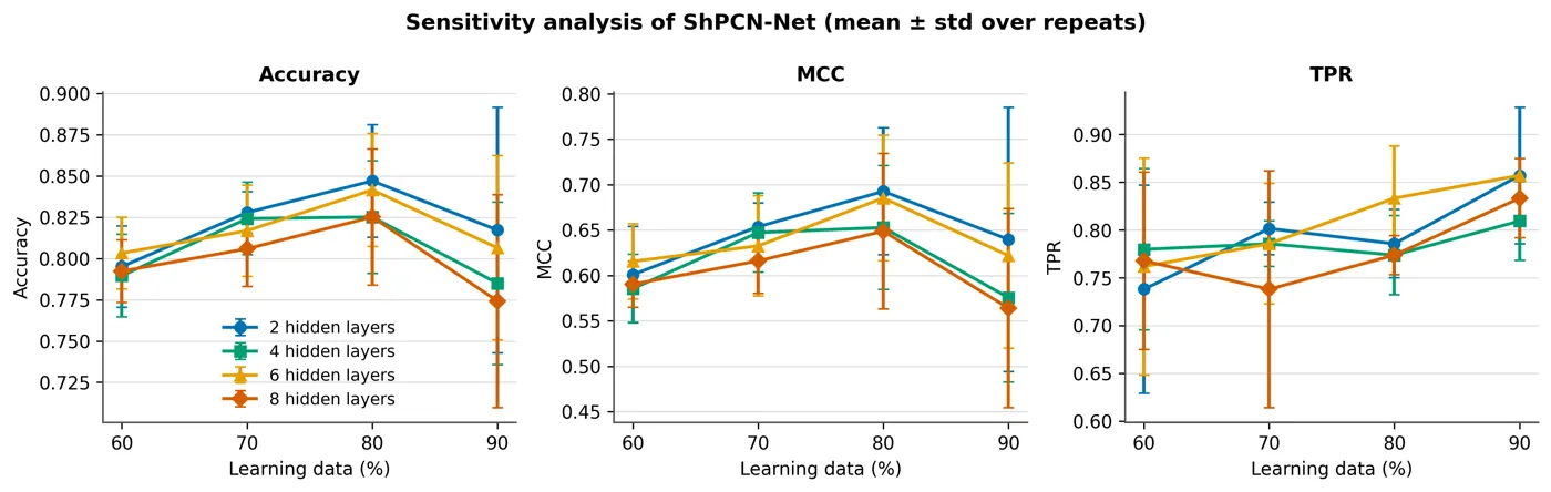
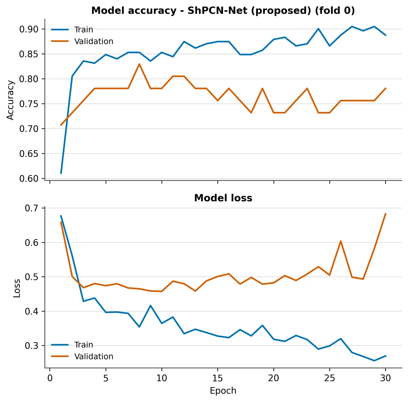
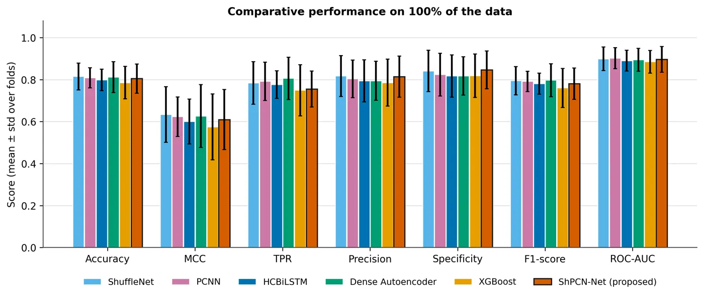
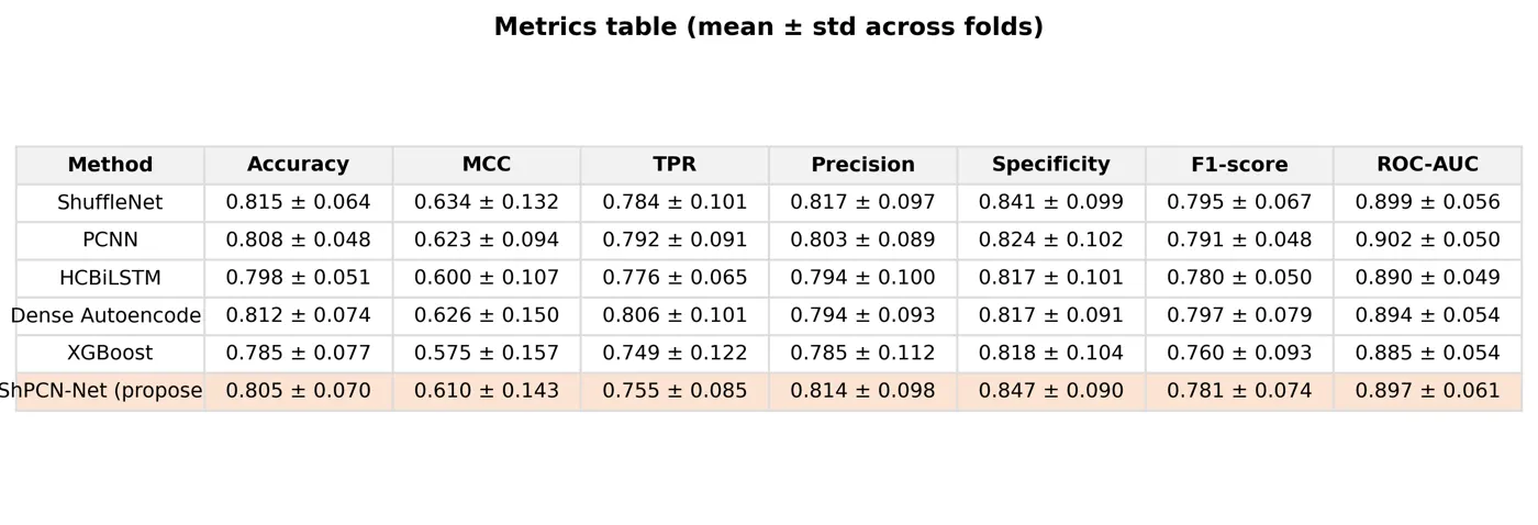
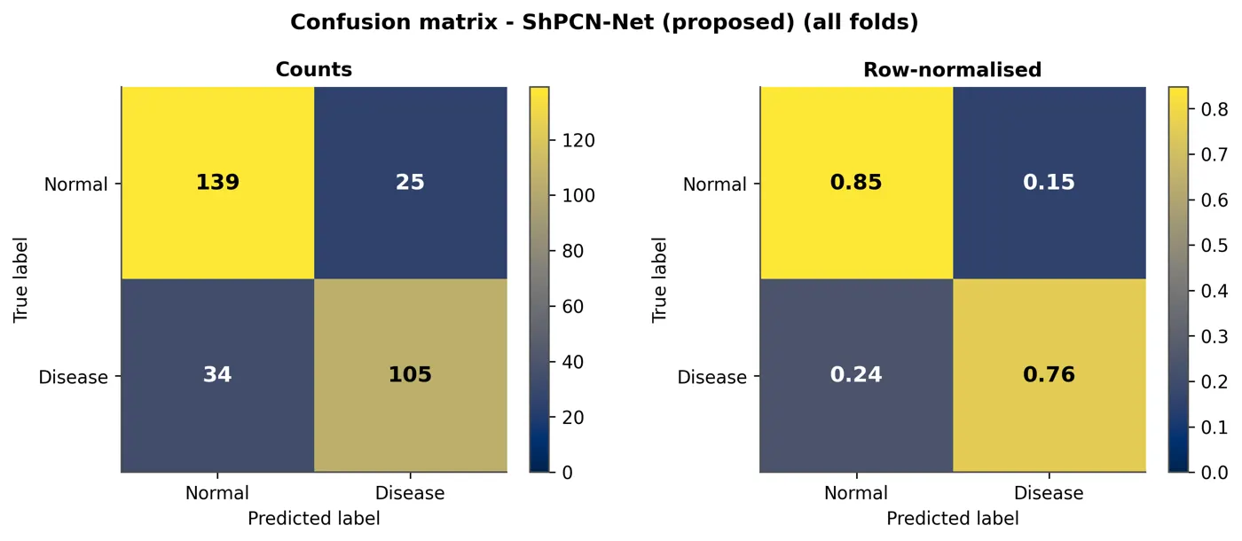
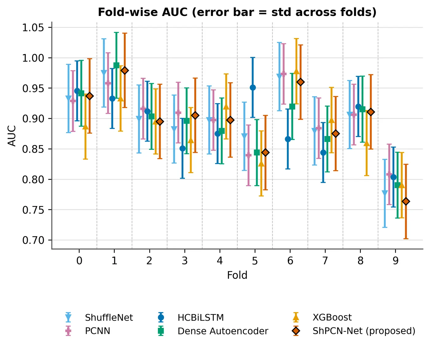
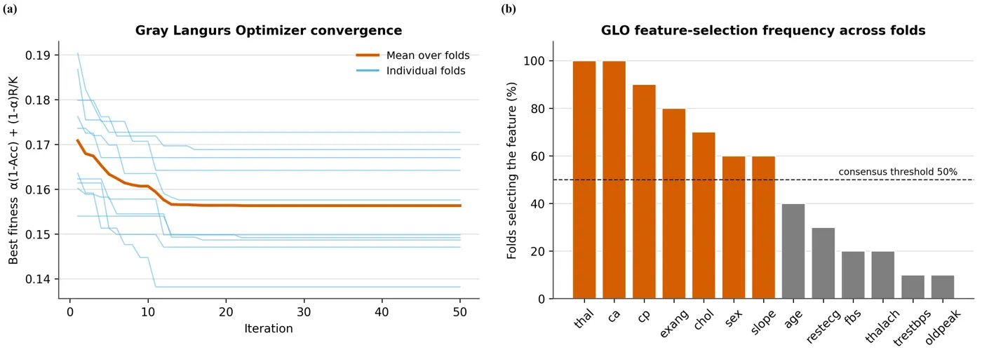
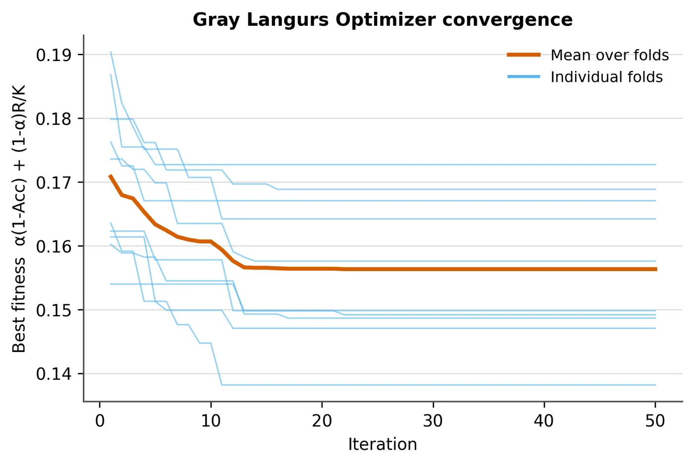
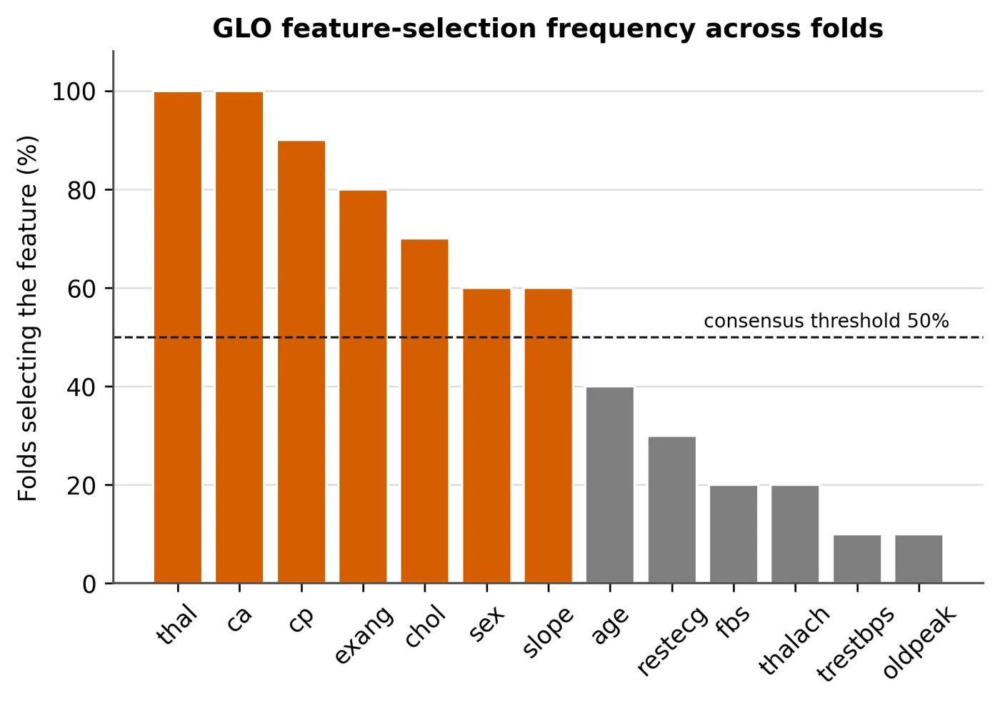
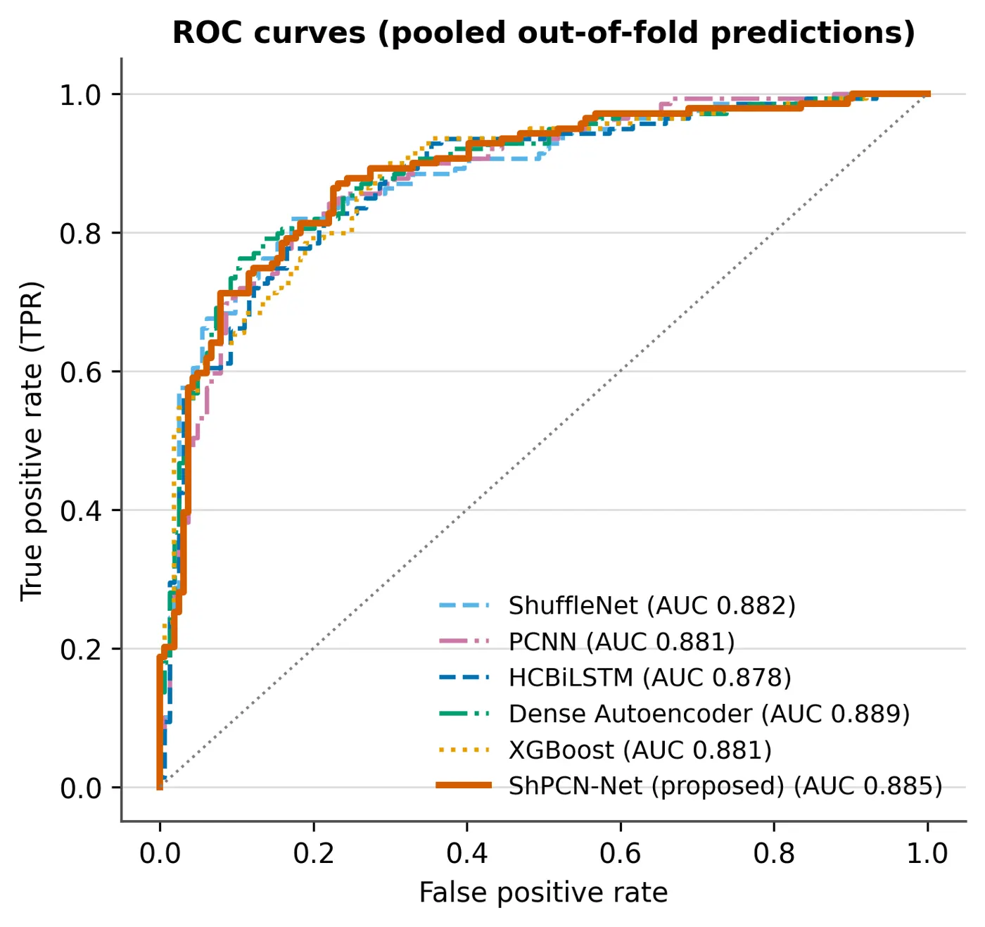
Every graph and diagram the run produced, grouped by purpose. Filter by group and click any graph to enlarge it.
- Delivered
- 22 graphs and diagrams, all shown
- Formats
- PNG, vector PDF and CSV for each
Loading the PDF… 0%
The manuscript as written, before any journal formatting, in a PDF viewer with page jump and zoom.
- Length
- 34 pages, before formatting
- Viewer
- Zoom, page jump, full screen, download
Loading the PDF… 0%
The final paper: the same manuscript typeset in the IEEE two-column layout, with figures placed and references formatted.
- Final paper
- 17 pages, IEEE two-column
- Word (DOCX)
- LaTeX source
Author names in the samples are placeholders.
Author names in the papers are placeholders. Samples show structure and are not published work.
The workflow
Six steps in one connected pipeline
One connected pipeline, not many disconnected AI tools. Each stage takes the approved output of the one before it, so nothing has to be copied, re-explained or rebuilt by hand. Open any stage to see what it does and what it needs from you.
You approve each step. EasySeer writes only the first draft.
Time and cost
Hours and dollars saved on one paper
Estimates for one journal article, stage by stage, comparing a researcher working across separate tools and paid support with the same work done in EasySeer.
| Research stage | Researcher + existing tools* | EasySeer* |
|---|---|---|
| Concept and novelty check | 10–20 hrs | 15–30 min |
| Code writing and debugging | 25–50 hrs | 30–90 min |
| Code execution and results | 15–30 hrs | 30 min–3 hrs |
| Manuscript writing | 30–50 hrs | 30–90 min |
| Formatting and delivery | 5–10 hrs | 10–30 min |
| Total | 105–200 hours | about 3–9 hours |
105–200 hours → about 3–9 hours*
Potentially save 100+ hours on a single research workflow.
| Research stage | External support cost* | EasySeer* |
|---|---|---|
| Concept and novelty check | $60–120 | Included |
| Code writing and debugging | $150–300 | Included |
| Code execution and results | $90–180 | Included |
| Manuscript writing | $200–450 | Included |
| Formatting and delivery | $40–90 | Included |
| Total | $630–$1,380 | $100 per project |
$630–$1,380 → $100 per project*
* Estimates for one journal article. They assume a researcher with moderate experience using several separate tools and, for cost, paid external support for each stage. These are EasySeer's own planning estimates, not independently measured results, and your own figures will differ.
The problem
Why one paper takes 105–200 hours
The time rarely goes into the science. It goes into the gaps between tools.
Scattered tools
One tool for notes, another for code, another for writing, another for formatting. Every hand-off means copying, re-explaining and fixing.
Late discovery
Weak ideas, missing baselines and journal mismatches are found months in, after the code and the draft are already written.
Untraceable results
Numbers in a draft drift away from the code that produced them, so every revision starts with detective work.
EasySeer keeps the whole research workflow in one project: the idea, the code, the results, the draft and the formatted delivery. You approve each step.
Compared
A connected workflow, not a pile of tools
General AI assistants are useful for many jobs. Here is how they usually fit this one.
Who it is for
Built for people who publish from code
From first-year scholars to whole research groups, EasySeer fits anyone who turns an idea, some code and some data into a paper.
PhD scholars
Several papers, one workflow. Test ideas early and keep every file together.
Read more →Master's students
Learn the research workflow by working through a real, structured project.
Read more →Postdocs and early-career researchers
Move ideas to first drafts faster while you juggle experiments and grants.
Read more →Research supervisors
See the reasoning behind a draft and discuss science instead of logistics.
Read more →Engineering and data science researchers
Keep code, logs, results and text together so numbers trace to files.
Read more →Universities and research groups
Give a whole group the same stepwise workflow and consistent AI disclosure.
Read more →Faculty and lecturers
Start papers from a scored concept between lectures.
Read more →Independent researchers
A structured workflow when you have no lab or team.
Read more →Industry R&D teams
Reproducible projects with data on your own computer.
Read more →Health and life-science researchers
Code-driven studies, documented step by step.
Read more →Researchers writing in a second language
A clear English draft from your own results.
Read more →Research offices and training centres
A visible workflow for training researchers.
Read more →Ethics first
Your ideas. Your authorship. Your approval.
EasySeer creates only an initial draft from the novel concept you provide, and it is designed to follow academic ethical guidelines.
- You stay the authorEasySeer produces a first draft. You verify, rewrite and decide. Authorship and accountability stay with you and your co-authors.
- No invented dataResults come from code that actually ran on your data. Weak results are reported as they are.
- Verify every referenceSuggested references must be checked by you. A citation is never proof that a claim is true.
- Disclose AI useMany journals and universities ask authors to declare AI assistance. EasySeer helps you prepare a disclosure statement. Follow the rules that apply to you.
- No promises about outcomesWe do not promise acceptance, a similarity score, or that detectors will or will not flag text.
- You approve each stepNothing moves forward without your approval, leaving a clear record of what you accepted.
Questions
Answers before you ask
The things scholars ask us first: what it does, what it costs and how it treats ethics and your data.
What is EasySeer?
EasySeer is an AI research-workflow tool. From your handwritten or typed concept it checks the idea, writes code, runs it, drafts a manuscript, formats it and delivers it to your project folder.
Who is EasySeer for?
Research scholars: PhD and master's students, postdocs and early-career researchers, plus supervisors and research groups.
Does EasySeer write my paper for me?
No. It creates only an initial draft from the novel concept you provide. You must verify the content, rewrite it in your own voice and take responsibility for the final paper.
Is using EasySeer ethical?
It is designed to follow academic ethical guidelines: it reports results as they are, does not invent data, asks for your approval at each step and supports an AI-use disclosure statement. Always follow your institution's and journal's rules on AI assistance.
Will EasySeer guarantee acceptance in a journal?
No. Acceptance is decided by editors and reviewers. EasySeer makes no promise of acceptance, ranking or any similarity score.
How much does it cost?
$100 per project for customers outside India, and Rs 10,000 per project in India. One credit runs one project.
Do credits expire?
No. Credits never expire.
What is the refund policy?
Payments are not refundable. If a project fails because of a fault on our side, the credit is restored, and a double or wrong charge is corrected. See the Refund policy.
Built for research at the top
The standard EasySeer is designed for
Scholars at the world's leading research universities work to a high bar for rigour and integrity. EasySeer is designed for that bar. It does not claim any partnership with the universities named here.
- United StatesMassachusetts Institute of Technology
- United KingdomImperial College London
- SwitzerlandETH Zurich
- SingaporeNational University of Singapore
- Hong Kong SARUniversity of Hong Kong
- AustraliaUNSW Sydney
- GermanyTechnical University of Munich
- CanadaMcGill University
- FranceUniversité PSL
- South KoreaSeoul National University
Turn your next handwritten concept into a first draft this week
Book a short demo, see a concept turn into a first draft and ask your questions. Pick the time.